Welcome

Deep Learning Notes
Notes taken during the Deep Learning Specialization
by Andrew Ng & Eddy Shyu
Stanford University & DeepLearning.AI
What I Built
| # | Course | Focus |
|---|---|---|
| 1 | Neural Networks and Deep Learning | Logistic regression as a neural network, shallow & deep networks, forward/backpropagation |
| 2 | Improving Deep Neural Networks | Hyperparameter tuning, regularization (Dropout, BatchNorm), optimization (Momentum, Adam), Xavier/He initialization |
| 3 | Structuring Machine Learning Projects | Train/dev/test splits, error analysis, transfer learning, end-to-end deep learning |
| 4 | Convolutional Neural Networks | CNNs, edge detection, classic & modern architectures (LeNet, AlexNet, VGG, ResNet, Inception, MobileNet, EfficientNet), object detection (YOLO), face recognition (FaceNet, Siamese), neural style transfer, U-Net |
| 5 | Sequence Models | RNNs, GRUs, LSTMs, word embeddings (Word2Vec, GloVe), attention models, Transformers, speech recognition, music synthesis, machine translation, chatbots |
— emreaslan —
Content
Welcome to Machine Learning notes.
∴
I completed the Machine Learning Specialization Course by taking detailed notes and summarizing critical concepts for future reference.
University of Stanford & DeepLearning.AI
— emreaslan —
Supervised and Unsupervised Machine Learning
Introduction
Machine learning is a branch of artificial intelligence that allows systems to learn and make predictions or decisions without explicit programming. Two main types of machine learning are Supervised Learning and Unsupervised Learning. Below is a summary of their characteristics, subfields, along with a visual representation for clarity.
graph TD
    A[Machine Learning] --> B[Supervised Learning]
    A --> C[Unsupervised Learning]
    B --> D[Regression]
    B --> E[Classification]
    C --> F[Clustering]
    C --> G[Association]
    C --> H[Dimensionality Reduction]
Supervised Learning
Supervised learning is a type of machine learning where the model is trained on labeled data. Labeled data means that each input has a corresponding output (or target) already provided. The goal is for the model to learn the relationship between the inputs and outputs so that it can make predictions for new, unseen data.
Key Characteristics
- Input and Output: The training data contains both input features (X) and target labels (Y).
- Goal: Predict the output (Y) for a given input (X).
Subfields
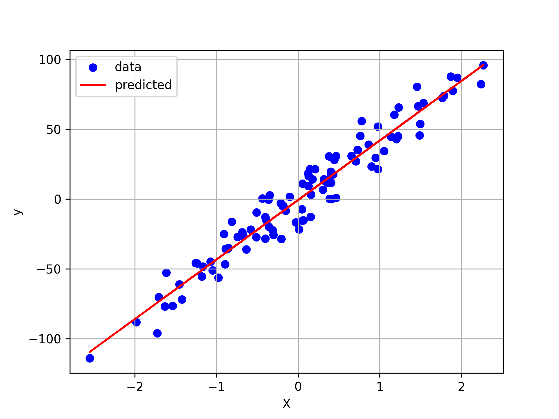
- Regression: Predicting continuous values (e.g., predicting rent prices based on apartment size).
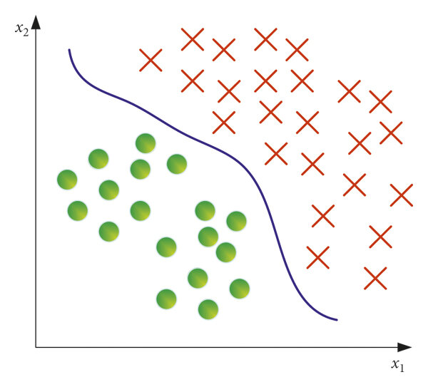
- Classification: Assigning inputs to discrete categories (e.g., diagnosing cancer as benign or malignant).
Example: Regression
- Scenario: Predicting rent prices based on apartment size (in m²).
- Details:
- Input features (X): Apartment size, number of rooms, neighborhood, etc.
- Target variable (Y): Rent price (e.g., $ per month).
- Model’s Job: Learn the relationship between apartment features and rent prices, then predict the rent for a new apartment.
Example: Classification
- Scenario: Diagnosing cancer (e.g., benign or malignant tumor).
- Details:
- Input features (X): Measurements like tumor size, texture, cell shape, etc.
- Target variable (Y): Class label (e.g., “Benign” or “Malignant”).
- Model’s Job: Classify a new tumor as benign or malignant based on input features.
Unsupervised Learning
Unsupervised learning deals with unlabeled data. The model tries to find patterns, structures, or relationships within the data without any predefined labels or targets. It’s often used for exploratory data analysis.
Key Characteristics
- Input Only: The data contains only input features (X), with no target labels (Y).
- Goal: Discover hidden patterns or groupings in the data.
Subfields
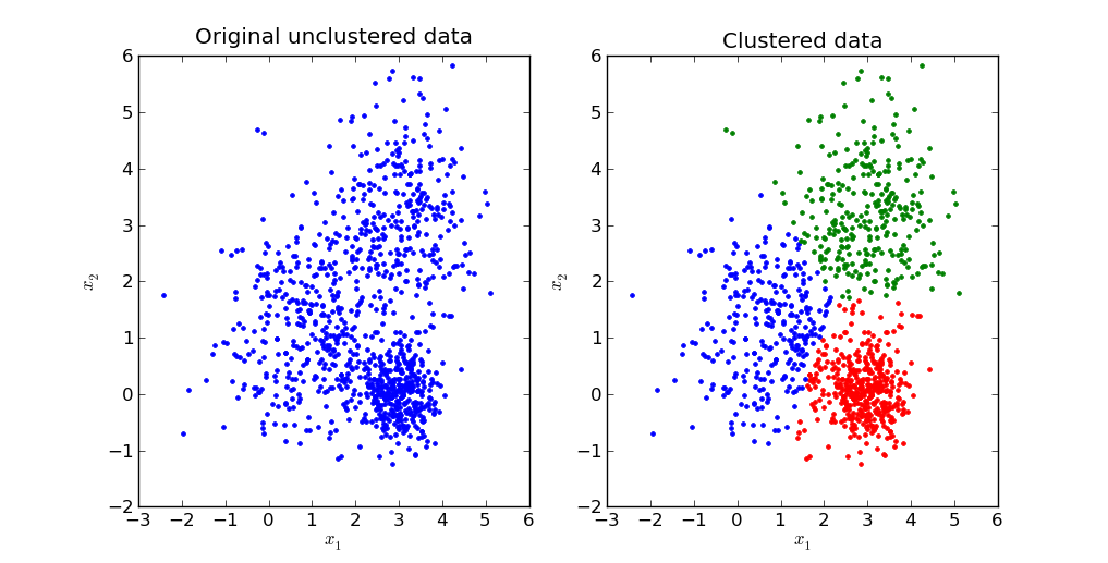
- Clustering: Grouping similar data points into clusters (e.g., customer segmentation).
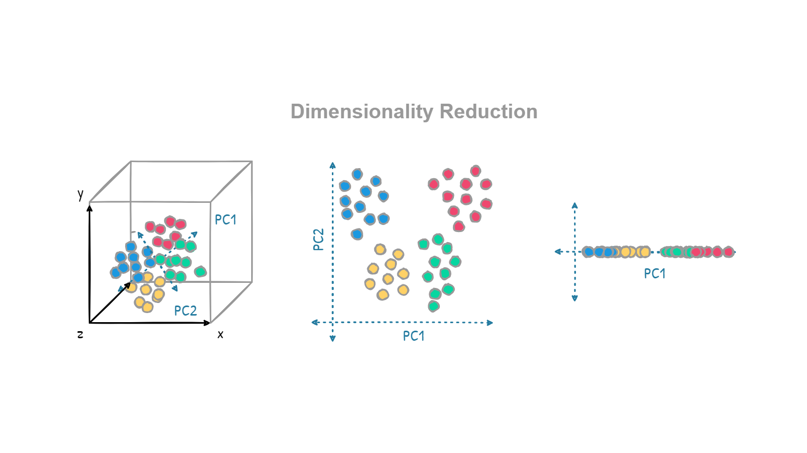
- Dimensionality Reduction: Reducing the number of features in the dataset while preserving important information (e.g., PCA).
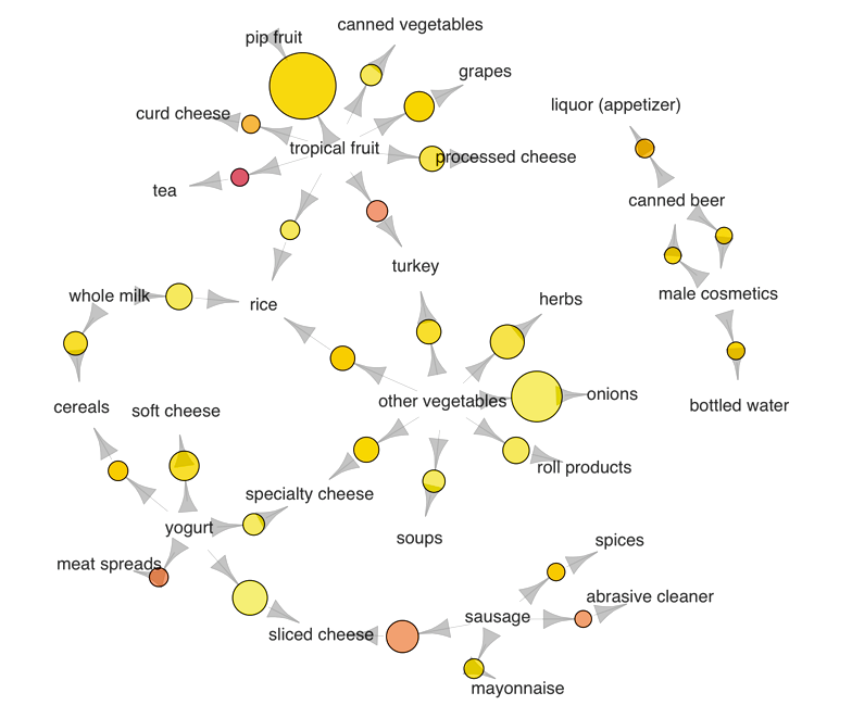
- Association: Discovering relationships or associations between variables in large datasets (e.g., market basket analysis).
Example: Clustering
- Scenario: Grouping customers for targeted marketing.
- Details:
- Input features (X): Customer age, income, purchase history, location, etc.
- No predefined labels (Y).
- Model’s Job: Identify clusters of customers (e.g., “High-spenders,” “Budget-conscious buyers”).
Example: Dimensionality Reduction
- Scenario: Visualizing high-dimensional data.
- Details:
- Imagine you have a dataset with 100+ features (e.g., sensor data from a factory).
- Dimensionality reduction (e.g., PCA) helps reduce it to 2D or 3D for easier visualization.
- Model’s Job: Keep the important structure of the data while reducing complexity.
Example: Association
- Scenario: Market basket analysis to identify product associations.
- Details:
- Input features (X): Transaction data showing items purchased together.
- No predefined labels (Y).
- Model’s Job: Identify rules like “If a customer buys bread, they are likely to buy butter.”
- Use Case: Recommendation systems, inventory planning.
Comparison Table
| Feature | Supervised Learning | Unsupervised Learning |
|---|---|---|
| Data Type | Labeled data (X, Y) | Unlabeled data (X only) |
| Goal | Predict outcomes | Find patterns or structures |
| Key Techniques | Regression, Classification | Clustering, Dimensionality Reduction, Assocation |
| Examples | Fraud detection, Stock price prediction | Market segmentation, Image compression |
Key Takeaways
- Supervised Learning requires labeled data and is commonly used for prediction tasks like regression and classification.
- Unsupervised Learning works with unlabeled data and focuses on finding hidden patterns through clustering or dimensionality reduction.
- Each technique has specific applications and is chosen based on the problem and the data available.
- Linear Regression and Cost Function
Linear Regression and Cost Function
1. Introduction
Linear regression is one of the fundamental algorithms in machine learning. It is widely used for predictive modeling, especially when the relationship between the input and output variables is assumed to be linear. The primary goal is to find the best-fitting line that minimizes the error between predicted values and actual values.
Why Linear Regression?
Linear regression is simple yet powerful for many real-world applications. Some common use cases include:
- Predicting house prices based on features like size, number of rooms, and location.
- Estimating salaries based on experience, education level, and industry.
- Understanding trends in various fields like finance, healthcare, and economics.
Real-World Example: Housing Prices
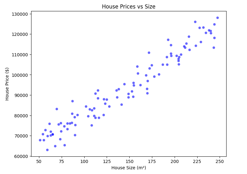
Consider predicting house prices based on the size of the house (in square meters). A simple linear relationship can be assumed: larger houses tend to have higher prices. This assumption is the foundation of our linear regression model.
2. Mathematical Representation
A simple linear regression model assumes a linear relationship between the input $x$ (house size in square meters) and the output $y$ (house price). It is represented as:
$$ h_θ(x) = \theta_0 + \theta_1 x $$
where:
- $h_θ(x) $ is the predicted house price.
- $ \theta_0 $ (intercept) and $\theta_1 $ (slope) are the parameters of the model.
- $x$ is the house size.
- $y$ is the actual house price.
2.1 Understanding the Linear Model
But what does this equation really mean?
-
$\theta_0$ (intercept): The price of a house when its size is 0 m².
-
$\theta_1$ (slope): The increase in house price for every additional square meter.
For example, if:
-
$\theta_0 = 50,000$ and $\theta_1 = 300$,
-
A 100 m² house would cost: $ h_θ(100) = 50000 + 300 \cdot 100 = 80000 $
-
A 200 m² house would cost: $ h_θ(200) = 50000 + 300 \cdot 200 = 110000 $
We can visualize this relationship using a regression line.
3. Implementing Linear Regression Step by Step
To make the theoretical concepts clearer, let’s implement the regression model step by step using Python.
3.1 Import Necessary Libraries
import numpy as np
import matplotlib.pyplot as plt
import seaborn as sns
3.2 Generate Sample Data
np.random.seed(42)
x = 50 + 200 * np.random.rand(100, 1)  # House sizes in m² (50 to 250)
y = 50000 + 300 * x + np.random.randn(100, 1) * 5000  # House prices with noise
Here, we create a dataset with 100 samples, where:
-
$x$ represents house sizes (random values between $50$ and $250$ m²).
-
$y$ represents house prices, following a linear relation but with some noise.
3.3 Visualizing the Data
plt.figure(figsize=(8,6))
sns.scatterplot(x=x.flatten(), y=y.flatten(), color='blue', alpha=0.6)
plt.xlabel('House Size (m²)')
plt.ylabel('House Price ($)')
plt.title('House Prices vs Size')
plt.show()
3.4 Plotting the Regression Line
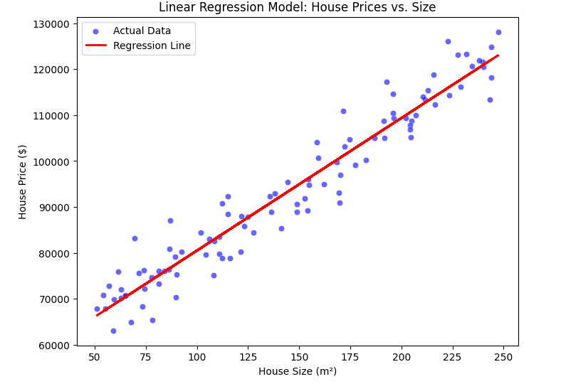
Before moving to cost function, let’s fit a simple regression line to our data and visualize it.
In real-world applications, we don’t manually compute these parameters. Instead, we use libraries like scikit-learn to perform linear regression efficiently.
3.4.1 Compute the Slope ($\theta_1$)
theta_1 = np.sum((x - np.mean(x)) * (y - np.mean(y))) / np.sum((x - np.mean(x))**2)
Here, we compute the slope ($\theta_1$) using the least squares method.
3.4.2 Compute the Intercept ($\theta_0$)
theta_0 = np.mean(y) - theta_1 * np.mean(x)
This calculates the intercept ($\theta_0$), ensuring that our regression line passes through the mean of the data.
3.5 Plotting the Regression Line
y_pred = theta_0 + theta_1 * x  # Compute predicted values

plt.figure(figsize=(8,6))
sns.scatterplot(x=x.flatten(), y=y.flatten(), color='blue', alpha=0.6, label='Actual Data')
plt.plot(x, y_pred, color='red', linewidth=2, label='Regression Line')
plt.xlabel('House Size (m²)')
plt.ylabel('House Price ($)')
plt.title('Linear Regression Model: House Prices vs. Size')
plt.legend()
plt.show()
3.6 Interpretation of the Regression Line
Now, what does this line tell us?
✅ If the slope $\theta_1$ is positive, then larger houses cost more (as expected).
✅ If the intercept $\theta_0$ is high, it means even the smallest houses have a significant base price.
✅ The steepness of the line shows how much price increases per square meter.
4. Cost Function
To measure how well our model is performing, we use the cost function. The most common cost function for linear regression is the Mean Squared Error (MSE):
$$ J(\theta) = \frac{1}{2m} \sum (h_{\theta}(x_i) - y_i)^2 $$
where:
- $ m $ is the number of training examples.
- $ h_\theta(x_i) $ is the predicted price for the $ i-th$ house.
- $ y_i $ is the actual price.
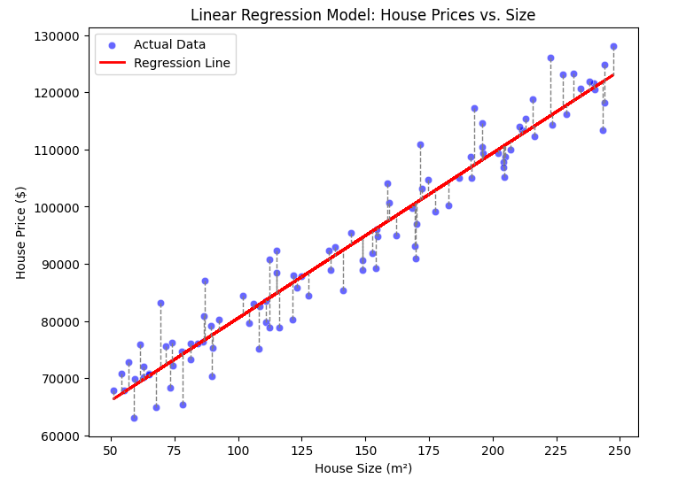
Any dashed line indicates an error. In the formula above, we calculated the sum of these, namely $J(\theta)$.
This function calculates the average squared difference between predicted and actual values, penalizing larger errors more. The goal is to minimize $J(\theta)$ to achieve the best model parameters.
4.1 Example: Assuming $\theta_1 = 0$
To illustrate how the cost function behaves, let’s assume that $\theta_1 = 0$, meaning our model only depends on $\theta_0$. We’ll use a small dataset with four x values and y values:
| x values | y values |
|---|---|
| 1 | 2 |
| 2 | 4 |
| 3 | 6 |
| 4 | 8 |
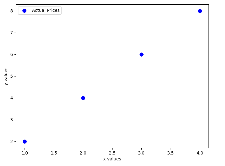
Since we assume $\theta_1 = 0$, our hypothesis function simplifies to: $$h_{\theta}(x) = \theta_0 \cdot x $$
We’ll evaluate different values of $\theta_0$ and compute the corresponding cost function.
Case 1: $\theta_0 = 1$
For $\theta_0 = 1$, the predicted values are:
$$ h_θ(x) = 1 \cdot x = [1, 2, 3, 4] $$
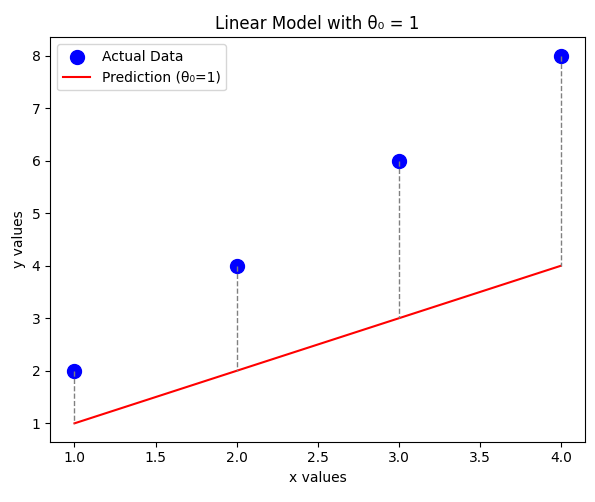
The error values:
$$ \text{error} = h_θ(x) - y = [1 - 2, 2 - 4, 3 - 6, 4 - 8] = [-1, -2, -3, -4] $$
Computing the cost function:
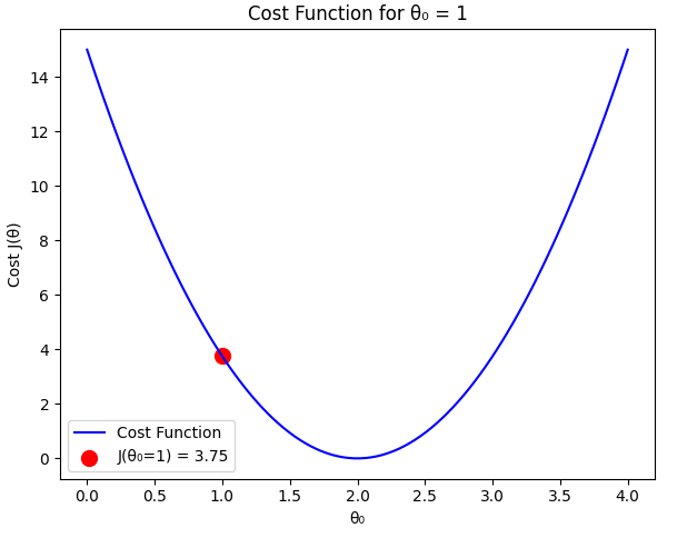
$$ J(\theta0 = 1) = \frac{1}{2m} \sum (h{\theta}(x_i) - y_i)^2 $$
$$ J(1) = \frac{1}{8} ((-1)^2 + (-2)^2 + (-3)^2 + (-4)^2) = \frac{1}{8} (1 + 4 + 9 + 16) = \frac{30}{8} = 3.75 $$
Case 2: $\theta_0 = 1.5$
For $\theta_0 = 1.5$, the predicted values are:
$$ h_θ(x) = 1.5 \cdot x = [1.5, 3, 4.5, 6] $$
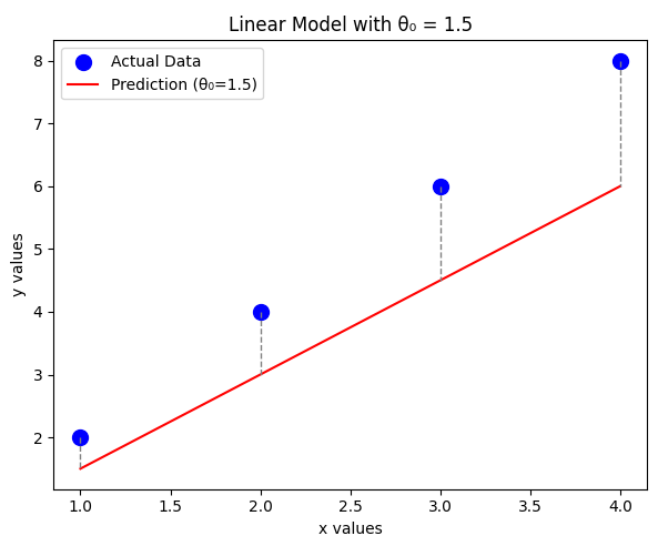
The error values:
$$ \text{error} = [1.5 - 2, 3 - 4, 4.5 - 6, 6 - 8] = [-0.5, -1, -1.5, -2] $$
Computing the cost function:
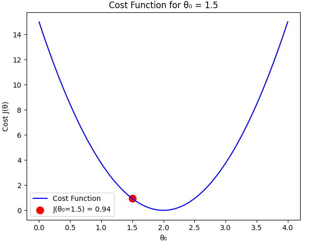
$$ J(1.5) = \frac{1}{8} ((-0.5)^2 + (-1)^2 + (-1.5)^2 + (-2)^2) $$
$$ J(1.5) = \frac{1}{8} (0.25 + 1 + 2.25 + 4) = \frac{7.5}{8} = 0.9375 $$
Case 3: $\theta_0 = 2$ (Optimal Case)
For $\theta_0 = 2$, the predicted values match the actual values:
$$ h_θ(x) = 2 \cdot x = [2, 4, 6, 8] $$
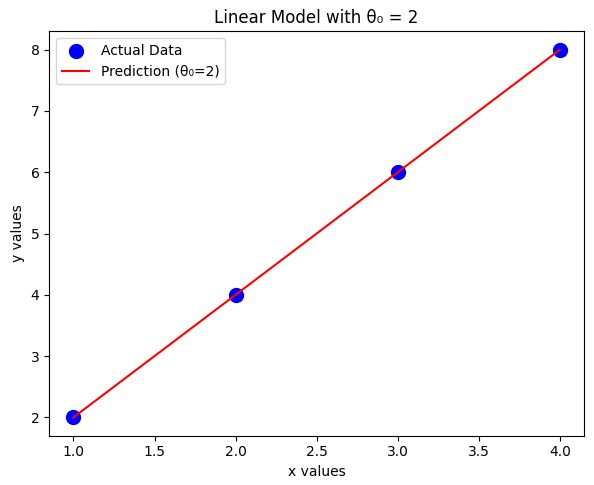
The error values:
$$ \text{error} = [2 - 2, 4 - 4, 6 - 6, 8 - 8] = [0, 0, 0, 0] $$
Computing the cost function:
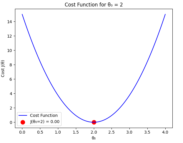
$$ J(2) = \frac{1}{8} ((0)^2 + (0)^2 + (0)^2 + (0)^2) = 0 $$
Comparison
From our calculations:
- $ J(1) = 3.75 $
- $ J(1.5) = 0.9375 $
- $ J(2) = 0 $
As expected, the cost function is minimized when $\theta_0 = 2$, which perfectly fits the dataset. Any deviation from this value results in a higher cost.
So how many times can the machine try and find the correct value? How can we teach it this? The answer is in the next topic.
Gradient Descent
- Introduction to Gradient Descent
- Mathematical Formulation of Gradient Descent
- Learning Rate ($\alpha$)
- Gradient Descent Convergence
- Local Minimum vs Global Minimum
Introduction to Gradient Descent
In the previous section, we explored how the cost function behaves when assuming different values of $\theta_0$ with $\theta_1 = 0$ (To visualize it easily, we give zero to $\theta_1$). Now, we introduce Gradient Descent, an optimization algorithm used to find the best parameters that minimize the cost function $J(\theta)$.
our hypothesis function simplifies to: $$h_{\theta}(x) = \theta_0 \cdot x $$
Gradient Descent is an iterative method that updates the parameter $\theta$ step by step in the direction that reduces the cost function. The algorithm helps us find the optimal value of $\theta_0$ efficiently instead of manually testing different values.
To understand how Gradient Descent works, let’s recall our dataset:
| x values | y values |
|---|---|
| 1 | 2 |
| 2 | 4 |
| 3 | 6 |
| 4 | 8 |
We aim to find the best value of $\theta_0$ that minimizes the error between our predictions $h_\theta(x) = \theta_0 \cdot x$ and the actual $y$ values. Gradient Descent will iteratively adjust $\theta_0$ to reach the minimum cost.
Mathematical Formulation of Gradient Descent
Gradient Descent is an optimization algorithm used to minimize a function by iteratively updating its parameters in the direction of the steepest descent. In our case, we aim to minimize the cost function:
$$ J(\theta) = \frac{1}{2m} \sum (h_θ(x_i) - y_i)^2 $$
Where:
- 𝑚 is the number of training examples.
- $h_θ(x)$ represents our hypothesis function (predicted values).
- y represents the actual target values.
- Goal: Find the optimal $θ$ that minimizes $J(θ)$.
1. Gradient Descent Update Rule
Gradient Descent uses the derivative of the cost function to determine the direction and magnitude of updates. The general update rule for $\theta$ is:
$$\theta := \theta - \alpha \frac{\partial J(\theta)}{\partial \theta}$$
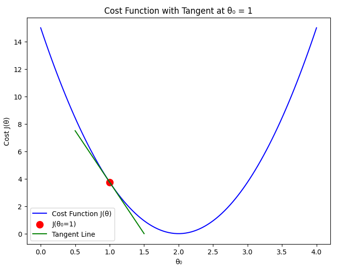
Where:
- $\alpha$ (learning rate) controls the step size of updates.
- $\frac{\partial J(\theta)}{\partial \theta} $ is the gradient (derivative) of the cost function with respect to $ \theta $.
Why Do We Use the Derivative?
The derivative $\frac{\partial J(\theta)}{\partial \theta} $ tells us the slope of the cost function. If the slope is positive, we need to decrease $θ_0$ , and if it is negative, we need to increase $θ_0$, guiding us toward the minimum of $J(θ_0)$ . Without derivatives, we wouldn’t know which direction to move to minimize the function.
The gradient tells us how steeply the function increases or decreases at a given point.
- If the gradient is positive, $ \theta $ is decreased.
- If the gradient is negative, $ \theta $ is increased.
This ensures that we move toward the minimum of the cost function.
2. Computing the Gradient
First, recall our hypothesis function:
$$ h_θ(x) = \theta_0 \cdot x $$
Now, we compute the derivative of the cost function:
$$ \frac{\partial J(\theta)}{\partial \theta*0} = \frac{1}{m} \sum (h_θ(x^{(i)}) - y^{(i)}) x^{(i)} $$
This expression represents the average gradient of the errors multiplied by the input values. Using this gradient, we update $ \theta_0 $ in each iteration:
$$ \theta*0 := \theta_0 - \alpha \cdot \frac{1}{m} \sum(h_θ(x^{(i)}) - y^{(i)}) x^{(i)} $$
- If the error is large, the update step is bigger.
- If the error is small, the update step is smaller.
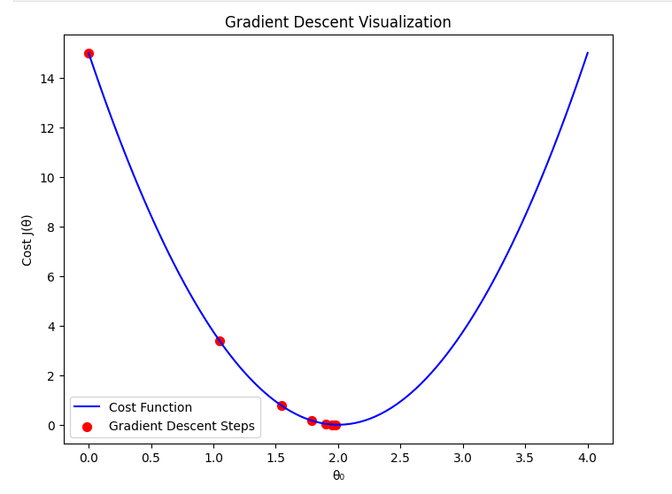
This way, the algorithm gradually moves towards the optimal $ \theta_0 $.
Learning Rate ($\alpha$)
The learning rate $(\alpha)$ is a crucial parameter in the gradient descent algorithm. It determines how large a step we take in the direction of the negative gradient during each iteration. Choosing an appropriate learning rate is essential for ensuring efficient convergence of the algorithm.
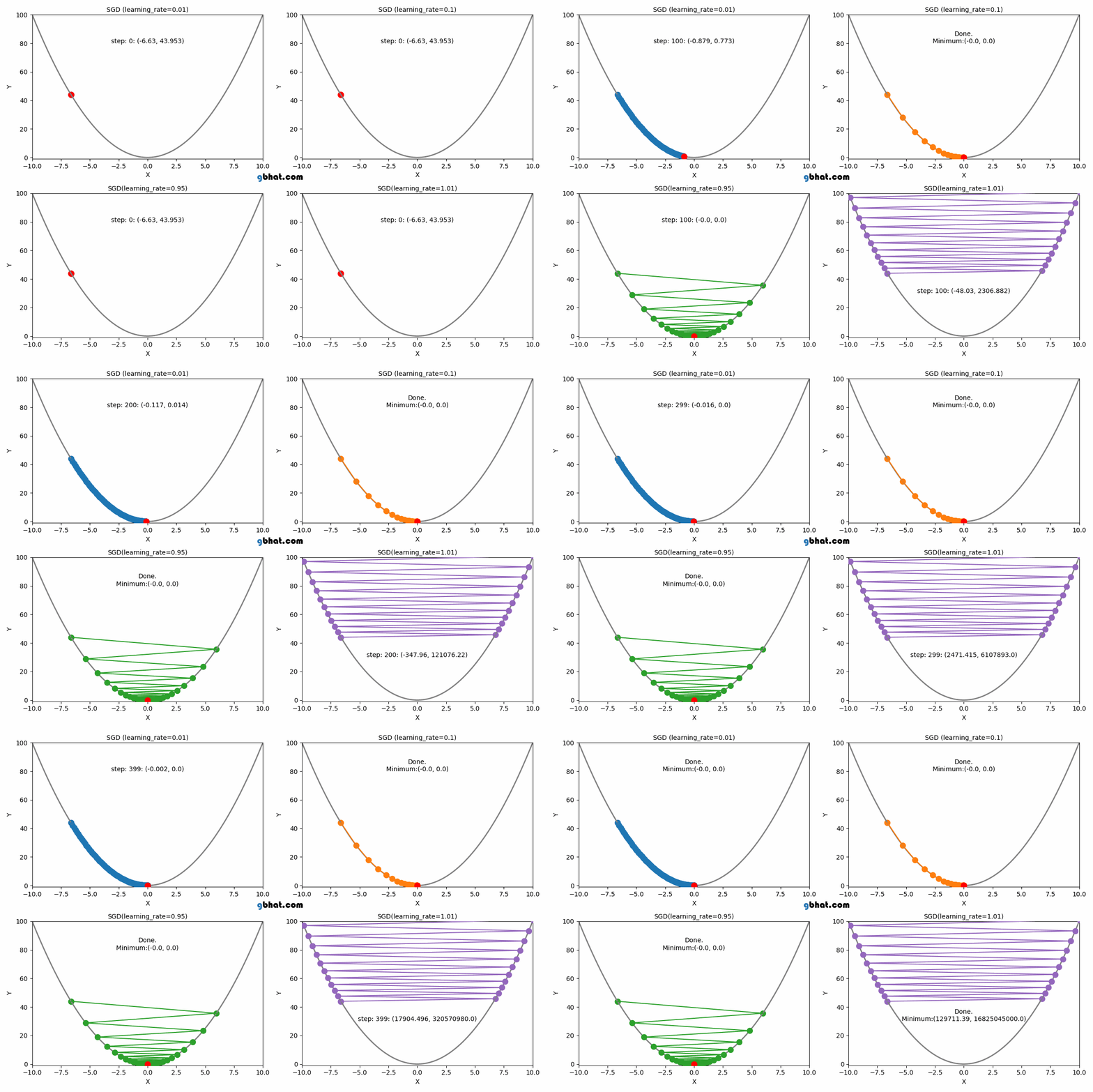
If the learning rate is too small, the algorithm will take tiny steps towards the minimum, leading to slow convergence. On the other hand, if the learning rate is too large, the algorithm may overshoot the minimum or even diverge, never reaching an optimal solution.
1. When $\alpha$ is Too Small
If the learning rate is set too small:
- Gradient descent will take very small steps in each iteration.
- Convergence to the minimum cost will be extremely slow.
- It may take a large number of iterations to reach a useful solution.
- The algorithm might get stuck in local variations of the cost function, slowing down learning.
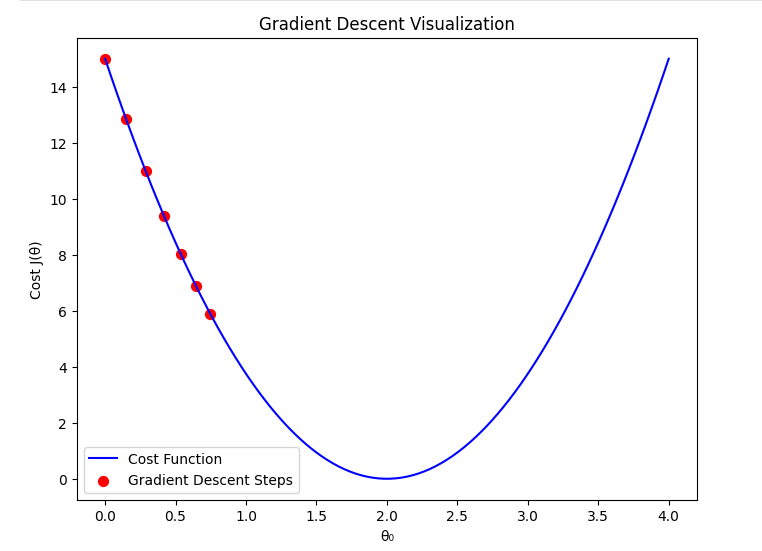
Mathematically, the update rule is: $\theta_0 := \theta_0 - \alpha \frac{d}{d\theta_0} J(\theta_0) $ When $\alpha$ is very small, the change in $\theta_0$ per step is minimal, making the process inefficient.
2. When $\alpha$ is Optimal
If the learning rate is chosen optimally:
- The gradient descent algorithm moves efficiently towards the minimum.
- It balances speed and stability, converging in a reasonable number of iterations.
- The cost function decreases steadily without oscillations or divergence.
A well-chosen $\alpha$ ensures that gradient descent follows a smooth and steady path to the minimum.
3. When $\alpha$ is Too Large
If the learning rate is set too large:
- Gradient descent may take excessively large steps.
- Instead of converging, it may oscillate around the minimum or diverge entirely.
- The cost function might increase instead of decreasing due to overshooting the optimal $\theta_0$.
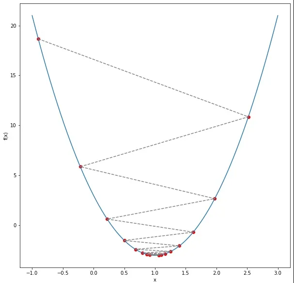
In extreme cases, the cost function values might increase indefinitely, causing the algorithm to fail to find a minimum.
Summary
Selecting the right learning rate is essential for gradient descent to work efficiently. A well-balanced $\alpha$ ensures that the algorithm converges quickly and effectively. In the next section, we will implement gradient descent with different learning rates to visualize their effects.
Gradient Descent Convergence
Gradient Descent is an iterative optimization algorithm that minimizes the cost function, J(\theta), by updating parameters step by step. However, we need a proper stopping criterion to determine when the algorithm has converged.
1. Convergence Criteria
The algorithm should stop when one of the following conditions is met:
- Small Gradient: If the derivative (gradient) of the cost function is close to zero, meaning the algorithm is near the optimal point.
- Minimal Cost Change: If the difference in the cost function between iterations is below a predefined threshold ($ |J(\thetat) - J(\theta{t-1})| < \varepsilon $).
- Maximum Iterations: A fixed number of iterations is reached to avoid infinite loops.
2. Choosing the Right Stopping Condition
- Stopping Too Early: If the algorithm stops before reaching the optimal solution, the model may not perform well.
- Stopping Too Late: Running too many iterations may waste computational resources without significant improvement.
- Optimal Stopping: The best condition is when further updates do not significantly change the cost function or parameters.
Local Minimum vs Global Minimum
Understanding the Concept
When optimizing a function, we aim to find the point where the function reaches its lowest value. This is crucial in machine learning because we want to minimize the cost function $ J(\theta) $ effectively. However, there are two types of minima that gradient descent might encounter:
- Global Minimum: The absolute lowest point of the function. Ideally, gradient descent should converge here.
- Local Minimum: A point where the function has a lower value than nearby points but is not the absolute lowest value.
For convex functions (such as our quadratic cost function), gradient descent is guaranteed to reach the global minimum. However, for non-convex functions, the algorithm may get stuck in a local minimum.
Convex vs Non-Convex Cost Functions
- Convex Functions
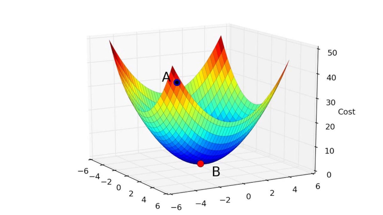
- The cost function $ J(\theta) $ is convex for linear regression.
- This ensures that gradient descent always leads to the global minimum.
- Example: A simple quadratic function like $ J(\theta) = (\theta - 2)^2 $.
- Non-Convex Functions
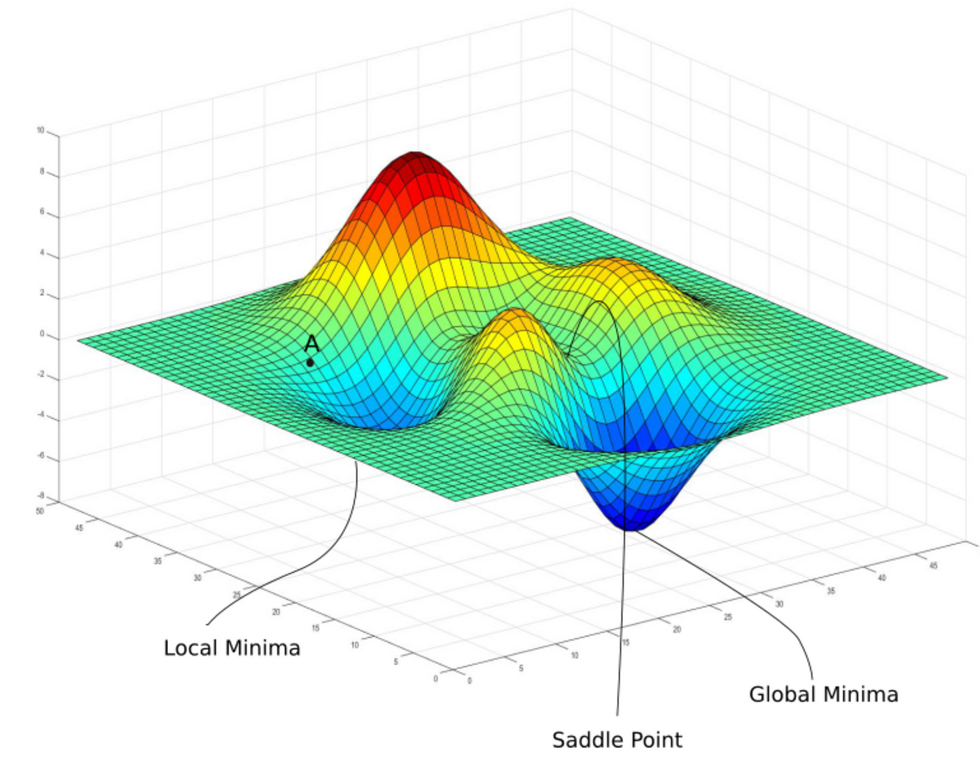
- More common in deep learning and complex machine learning models.
- There can be multiple local minima.
- Example: Functions with multiple peaks and valleys, such as $J(\theta) = \sin(\theta) + \frac{\theta^2}{10} $.
Multiple Features
Introduction
In real-world scenarios, a single feature is often not enough to make accurate predictions. For example, if we want to predict the price of a house, using only its size (square meters) might not be sufficient. Other factors such as the number of bedrooms, location, and age of the house also play an important role.
When we have multiple features, our hypothesis function extends to:
$$ h_{\theta}(x) = \theta_0 + \theta_1 x_1 + \theta_2 x_2 + … + \theta_n x_n $$
where:
- $ x_1, x_2, …, x_n $ are the input features,
- $ \theta_0, \theta_1, …, \theta_n $ are the parameters (weights) we need to learn.
For instance, in a house price prediction model, the hypothesis function could be:
$$ h_{\theta}(x) = \theta_0 + \theta_1 (\text{Size}) + \theta_2 (\text{Number of Bedrooms}) + \theta_3 (\text{Age of House}) $$
This allows our model to consider multiple factors, improving its accuracy compared to using a single feature.
Vectorization
To optimize computations, we represent our hypothesis function using matrix notation:
where:
$ X $ is the matrix containing training examples
$ \theta $ is the parameter vector
This allows efficient computation using matrix operations instead of looping over individual training examples.
Why Vectorization?
Vectorization is the process of converting operations that use loops into matrix operations. This improves computational efficiency, especially when working with large datasets. Instead of computing predictions one by one using a loop, we leverage linear algebra to perform all calculations simultaneously.
Without vectorization (using a loop):
m = len(X)  # Number of training examples
h = []
for i in range(m):
    prediction = theta_0 + theta_1 * X[i, 1] + theta_2 * X[i, 2] + ... + theta_n * X[i, n]
    h.append(prediction)
With vectorization:
h = np.dot(X, theta) # Compute all predictions at once
This method is significantly faster because it takes advantage of optimized numerical libraries like NumPy that execute matrix operations efficiently.
Vectorized Cost Function
Similarly, our cost function for multiple features is:
$$ J(\theta) = \frac{1}{2m} \sum(h_θ(x^{(i)}) - y^{(i)})^2 $$
Using matrices, this can be written as:
$$ J(\theta) = \frac{1}{2m} (X\theta - y)^T (X\theta - y) $$
And implemented in Python as:
def compute_cost(X, y, theta):
    m = len(y)  # Number of training examples
    error = np.dot(X, theta) - y  # Compute (Xθ - y)
    cost = (1 / (2 * m)) * np.dot(error.T, error)  # Compute cost function
    return cost
By using vectorized operations, we achieve a significant performance boost compared to using explicit loops.
Feature Scaling
When working with multiple features, the range of values across different features can vary significantly. This can negatively affect the performance of gradient descent, causing slow convergence or inefficient updates. Feature scaling is a technique used to normalize or standardize features to bring them to a similar scale, improving the efficiency of gradient descent.
Why Feature Scaling is Important
- Features with large values can dominate the cost function, leading to inefficient updates.
- Gradient descent converges faster when features are on a similar scale.
- Helps prevent numerical instability when computing gradients.
Methods of Feature Scaling
1. Min-Max Scaling (Normalization)
Brings all feature values into a fixed range, typically between 0 and 1:
$$x^{(i)}{scaled} = \frac{x^{(i)} - x{min}}{x_{max} - x_{min}}$$
- Best for cases where the distribution of data is not Gaussian.
- Sensitive to outliers, as extreme values affect the range.
2. Standardization (Z-Score Normalization)
Centers data around zero with unit variance:
$$x^{(i)}_{scaled} = \frac{x^{(i)} - \mu}{\sigma}$$
where:
-
$ \mu $ is the mean of the feature values
-
$ \sigma $ is the standard deviation
-
Works well when features follow a normal distribution.
-
Less sensitive to outliers compared to min-max scaling.
Example
Consider a dataset with two features: House Size (m²) and Number of Bedrooms.
| House Size (m²) | Bedrooms |
|---|---|
| 2100 | 3 |
| 1600 | 2 |
| 2500 | 4 |
| 1800 | 3 |
Using min-max scaling:
| House Size (scaled) | Bedrooms (scaled) |
|---|---|
| 0.714 | 0.5 |
| 0.0 | 0.0 |
| 1.0 | 1.0 |
| 0.286 | 0.5 |
Feature Scaling in Gradient Descent
After scaling, gradient descent updates will be more balanced across different features, leading to faster and more stable convergence. Feature scaling is a critical preprocessing step in machine learning models involving optimization algorithms like gradient descent.
Feature Engineering and Polynomial Regression
- Feature Engineering
- Polynomial Regression
Feature Engineering
Introduction to Feature Engineering
Feature engineering is the process of transforming raw data into meaningful features that improve the predictive power of machine learning models. It involves creating new features, modifying existing ones, and selecting the most relevant features to enhance model performance.
Why is Feature Engineering Important?
- Improves model accuracy: Well-engineered features help models learn better representations of the data.
- Reduces model complexity: Properly engineered features can make complex models simpler and more interpretable.
- Enhances generalization: Good feature selection prevents overfitting and improves performance on unseen data.
Real-World Example
Consider a house price prediction problem. Instead of using just raw data such as square footage and the number of bedrooms, we can create new features like:
- Price per square foot =
Price / Size - Age of the house =
Current Year - Year Built - Proximity to city center =
Distance in km
These engineered features often provide better insights and improve model performance compared to using raw data alone.
Feature Transformation
Feature transformation involves applying mathematical operations to existing features to make data more suitable for machine learning models.
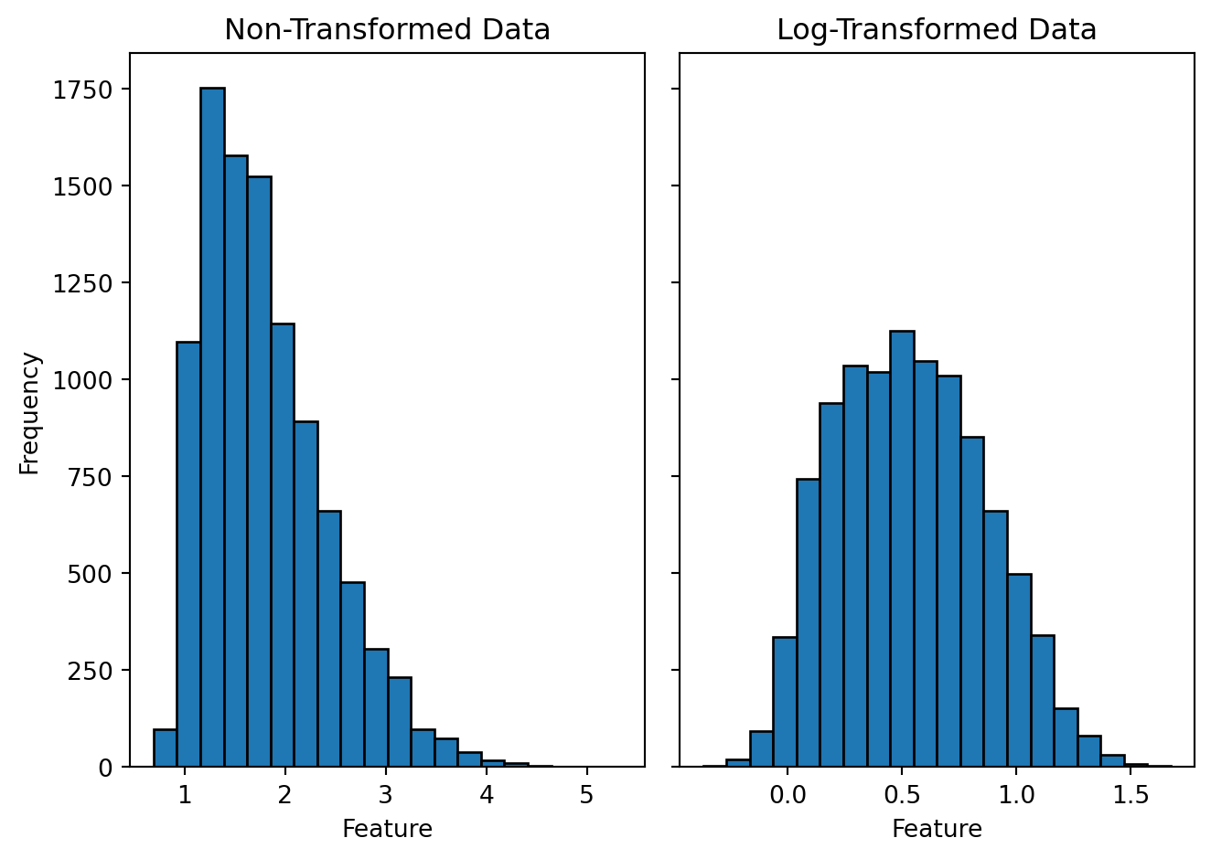
1. Log Transformation
Used to reduce skewness and stabilize variance in highly skewed data.
Example: Income Data
Many income datasets have a right-skewed distribution where most values are low, but a few values are extremely high. Applying a log transformation makes the data more normal:
$$X’ = \log(X)$$
2. Polynomial Features
Adding polynomial terms (squared, cubic) to capture non-linear relationships.
Example: House Price Prediction
Instead of using Size as a single feature, we can include Size^2 and Size^3 to better fit non-linear patterns.
from sklearn.preprocessing import PolynomialFeatures
import numpy as np

X = np.array([[1000], [1500], [2000], [2500]])  # House sizes
poly = PolynomialFeatures(degree=2)
X_poly = poly.fit_transform(X)
print(X_poly)
3. Interaction Features
Creating new features based on interactions between existing ones.
Example: Combining Features
Instead of using Height and Weight separately for a health model, create a new BMI feature:
$$BMI = \frac{Weight}{Height^2}$$
def calculate_bmi(height, weight):
    return weight / (height ** 2)

height = np.array([1.65, 1.75, 1.80])  # Heights in meters
weight = np.array([65, 80, 90])  # Weights in kg
bmi = calculate_bmi(height, weight)
print(bmi)
This allows the model to understand health risks better than using height and weight separately.
Feature Selection
Feature selection involves identifying the most relevant features for a model while removing unnecessary or redundant ones. This improves model performance and reduces computational complexity.
1. Unnecessary Features
Not all features contribute equally to model performance. Some may be irrelevant or redundant, leading to overfitting and increased computational cost. Examples of unnecessary features include:
- ID columns: Unique identifiers that do not provide predictive value.
- Highly correlated features: Features that contain similar information.
- Constant or near-constant features: Features with little to no variation.
2. Correlation Analysis
Correlation analysis helps detect multicollinearity, where two or more features are highly correlated. If two features provide similar information, one of them can be removed.
Example: Finding Highly Correlated Features
import pandas as pd
import numpy as np

# Sample dataset
data = {
    'Feature1': [1, 2, 3, 4, 5],
    'Feature2': [2, 4, 6, 8, 10],
    'Feature3': [5, 3, 6, 9, 2]
}
df = pd.DataFrame(data)

# Compute correlation matrix
correlation_matrix = df.corr()
print(correlation_matrix)
Features with a correlation coefficient close to ±1 can be considered redundant and removed.
3. Statistical Feature Selection Methods
Feature selection techniques can be used to rank the importance of different features based on statistical tests or model-based importance measures.
At this stage it is enough to learn superficially !
Common Methods:
- Chi-Square Test: Measures dependency between categorical features and the target variable.
- Mutual Information: Evaluates how much information a feature contributes.
- Recursive Feature Elimination (RFE): Iteratively removes less important features based on model performance.
- Feature Importance from Tree-Based Models: Decision trees and random forests provide feature importance scores.
Feature selection ensures that only the most valuable features are used in the final model, improving efficiency and predictive power.
Polynomial Regression
Introduction to Polynomial Regression
Polynomial Regression is an extension of Linear Regression that models non-linear relationships between input features and the target variable. While Linear Regression assumes a straight-line relationship, Polynomial Regression captures curves and more complex patterns.
Why Use Polynomial Regression?
- Handles Non-Linearity: Unlike Linear Regression, which assumes a direct relationship, Polynomial Regression models curved trends.
- Better Fit for Real-World Data: Many real-world phenomena, such as population growth, economic trends, and physics-based models, exhibit non-linear behavior.
- Feature Engineering Alternative: Instead of manually creating interaction terms, Polynomial Regression provides an automatic way to capture complex dependencies.
Example: Predicting House Prices
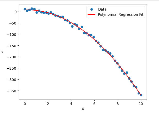
Consider a dataset where house prices do not increase linearly with size. Instead, they follow a non-linear trend due to factors like demand, location, and infrastructure. A Polynomial Regression model can better capture this pattern.
For instance:
- Linear Model: $ Price = \beta_0 + \beta_1 \cdot Size $
- Polynomial Model: $ Price = \beta_0 + \beta_1 \cdot Size + \beta_2 \cdot Size^2 $
This quadratic term helps model the curved price trend more accurately.
Mathematical Representation and Implementation
Polynomial regression extends linear regression by adding polynomial terms to the feature set. The hypothesis function is represented as:
$$ h_{\theta}(x) = \theta_0 + \theta_1 x + \theta_2 x^2 + \theta_3 x^3 + … + \theta_n x^n $$
where:
- $ x $ is the input feature,
- $ \theta_0, \theta_1, …, \theta_n $ are the parameters (weights),
- $ x^n $ represents higher-degree polynomial terms.
This allows the model to capture non-linear relationships in the data.
Classification with Logistic Regression
- 1. Introduction to Classification
- 2. Logistic Regression
- 3. Cost Function for Logistic Regression
- 4. Gradient Descent for Logistic Regression
1. Introduction to Classification
Classification is a supervised learning problem where the goal is to predict discrete categories instead of continuous values. Unlike regression, which predicts numerical values, classification assigns data points to labels or classes.
Classification vs. Regression
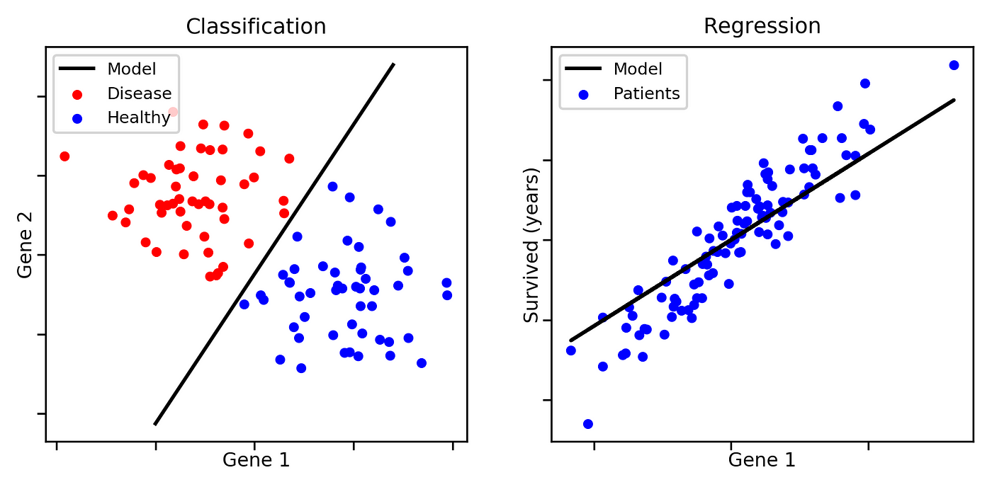
| Feature | Regression | Classification |
|---|---|---|
| Output Type | Continuous | Discrete |
| Example | Predicting house prices | Email spam detection |
| Algorithm Example | Linear Regression | Logistic Regression |
Examples of Classification Problems
- Email Spam Detection: Classify emails as “spam” or “not spam”.
- Medical Diagnosis: Identify whether a patient has a disease (yes/no).
- Credit Card Fraud Detection: Determine if a transaction is fraudulent or legitimate.
- Image Recognition: Classifying images as “cat” or “dog”.
Classification models can be:
- Binary Classification: Only two possible outcomes (e.g., spam or not spam).
- Multi-class Classification: More than two possible outcomes (e.g., classifying handwritten digits 0-9).
2. Logistic Regression
Introduction to Logistic Regression
Logistic regression is a statistical model used for binary classification problems. Unlike linear regression, which predicts continuous values, logistic regression predicts probabilities that map to discrete class labels.
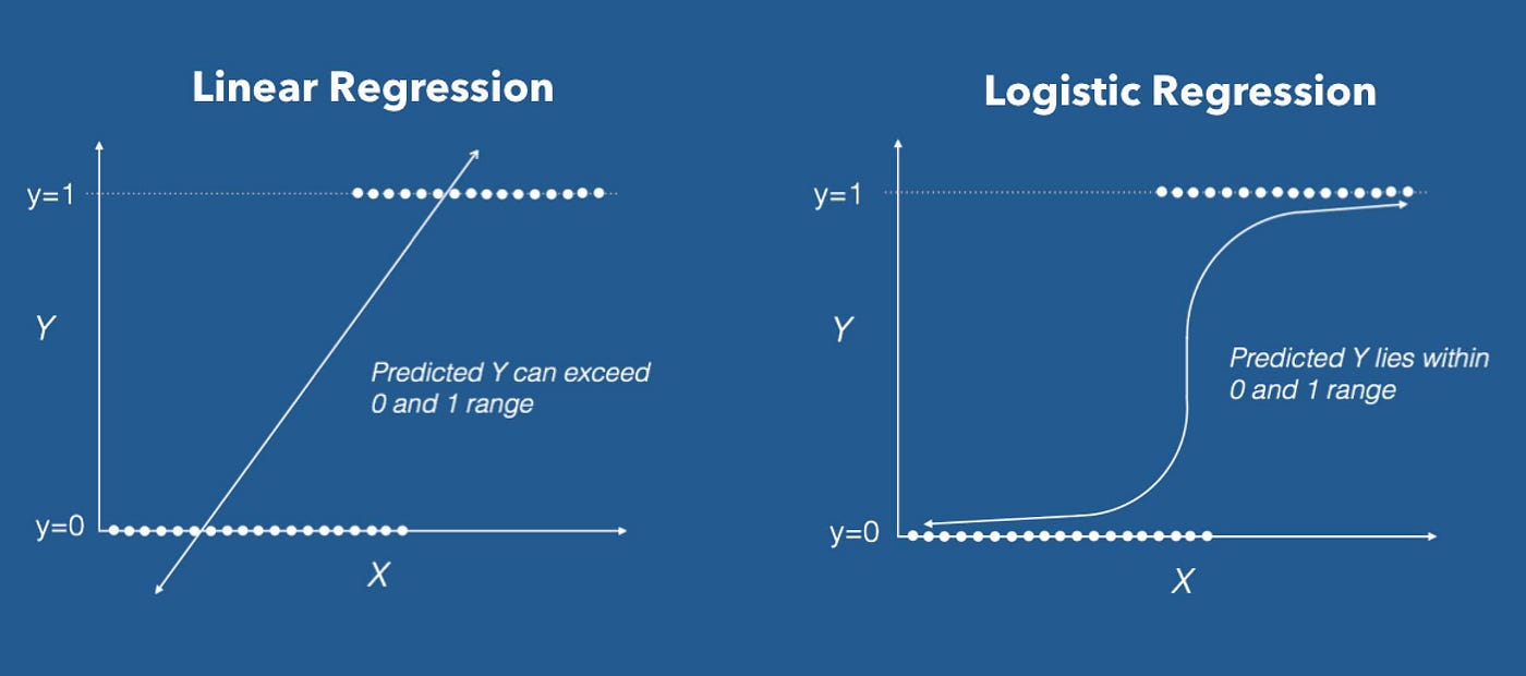
Linear regression might seem like a reasonable approach for classification, but it has major limitations:
- Unbounded Output: Linear regression produces outputs that can take any real value, meaning predictions could be negative or greater than 1, which makes no sense for probability-based classification.
- Poor Decision Boundaries: If we use a linear function for classification, extreme values in the dataset can distort the decision boundary, leading to incorrect classifications.
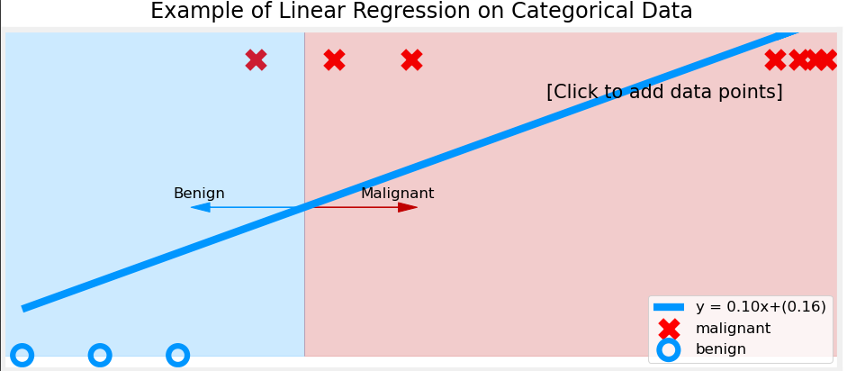
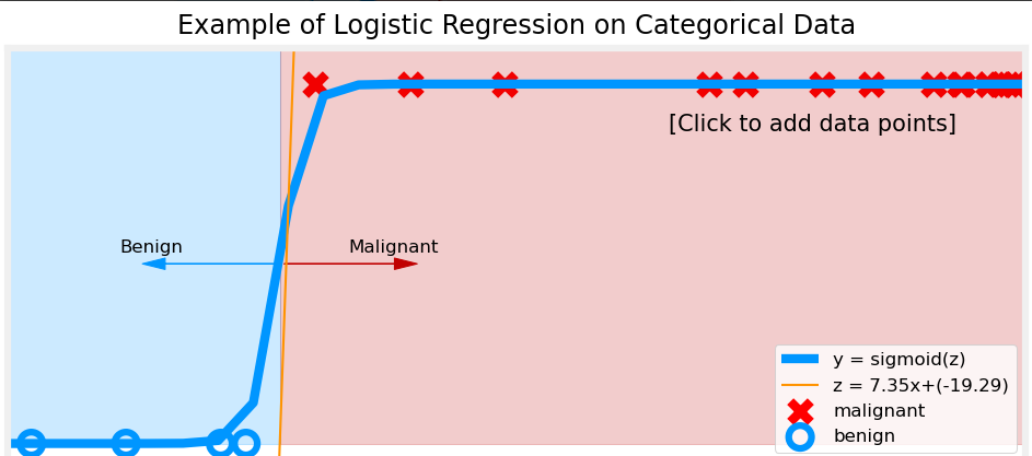
To solve these issues, we use logistic regression, which applies the sigmoid function to transform outputs into a probability range between 0 and 1.
Why Do We Need the Sigmoid Function?
The sigmoid function is a key component of logistic regression. It ensures that outputs always remain between 0 and 1, making them interpretable as probabilities.
Consider a fraud detection system that predicts whether a transaction is fraudulent (1) or legitimate (0) based on customer behavior. Suppose we use a linear model:
$$ y = \theta_0 + \theta_1 x_1 + \theta_2 x_2 $$
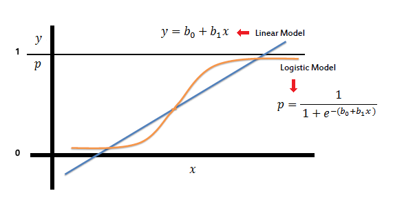
For some transactions, the output might be y = 7.5 or y = -3.2, which do not make sense as probability values. Instead, we use the sigmoid function to squash any real number into a valid probability range:
$$ h_{\theta}(x) = \frac{1}{1 + e^{-\theta^T x}} $$
This function maps:
- Large positive values to probabilities close to 1 (fraudulent transaction).
- Large negative values to probabilities close to 0 (legitimate transaction).
- Values near 0 to probabilities near 0.5 (uncertain classification).
Sigmoid Function and Probability Interpretation
The output of the sigmoid function can be interpreted as:
- $ h_θ(x) \approx 1 $ → The model predicts Class 1 (e.g., spam email, fraudulent transaction).
- $ h_θ(x) \approx 0 $ → The model predicts Class 0 (e.g., not spam email, legitimate transaction).
For a final classification decision, we apply a threshold (typically 0.5):
$$ \hat{y} = \begin{cases} 1, & \text{if } h_{\theta}(x) \geq 0.5 \ 0, & \text{if } h_{\theta}(x) < 0.5 \end{cases} $$
This means:
- If the probability is ≥ 0.5, we classify the input as 1 (positive class).
- If the probability is < 0.5, we classify it as 0 (negative class).
Decision Boundary
The decision boundary is the surface that separates different classes in logistic regression. It is the point at which the model predicts a probability of 0.5, meaning the model is equally uncertain about the classification.
Since logistic regression produces probabilities using the sigmoid function, we define the decision boundary mathematically as:
$$ h_{\theta}(x) = \frac{1}{1 + e^{-\theta^T x}} = 0.5 $$
Taking the inverse of the sigmoid function, we get:
$$ \theta^T x = 0 $$
This equation defines the decision boundary as a linear function in the feature space.
Understanding the Decision Boundary with Examples
1. Single Feature Case (1D)
If we have only one feature $ x_1 $, the model equation is:
$$ \theta_0 + \theta_1 x_1 = 0 $$
Solving for $ x_1 $:
$$ x_1 = -\frac{\theta_0}{\theta_1} $$
This means that when $ x_1 $ crosses this threshold, the model switches from predicting Class 0 to Class 1.
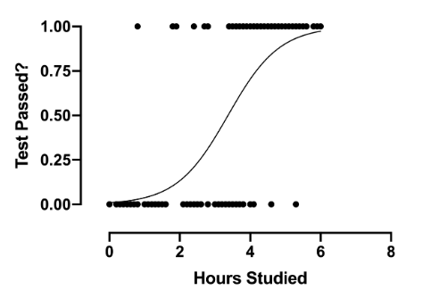
Example: Imagine predicting whether a student passes or fails based on study hours ($ x_1 $):
- If $ x_1 < 5 $ hours → Fail (Class 0).
- If $ x_1 \geq 5 $ hours → Pass (Class 1).
The decision boundary in this case is simply $ x_1 = 5 $.
2. Two Features Case (2D)
For two features $ x_1 $ and $ x_2 $, the decision boundary equation becomes:
$$ \theta_0 + \theta_1 x_1 + \theta_2 x_2 = 0 $$
Rearranging:
$$ x_2 = -\frac{\theta_0}{\theta_2} - \frac{\theta_1}{\theta_2} x_1 $$
This represents a straight line separating the two classes in a 2D plane.
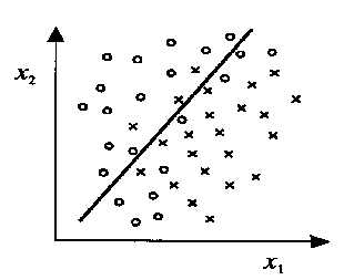
Example: Suppose we classify students as passing (1) or failing (0) based on study hours ($ x_1 $) and sleep hours ($ x_2 $):
- The decision boundary could be: $$ x_2 = -2 - 0.5 x_1 $$
- If $ x_2 $ is above the line, classify as pass.
- If $ x_2 $ is below the line, classify as fail.
3. Two Features Case (3D)
When we move to three features $ x_1 $, $ x_2 $, and $ x_3 $, the decision boundary becomes a plane in three-dimensional space:
$$ \theta_0 + \theta_1 x_1 + \theta_2 x_2 + \theta_3 x_3 = 0 $$
Rearranging for $ x_3 $:
$$ x_3 = -\frac{\theta_0}{\theta_3} - \frac{\theta_1}{\theta_3} x_1 - \frac{\theta_2}{\theta_3} x_2 $$
This equation represents a flat plane dividing the 3D space into two regions, one for Class 1 and the other for Class 0.
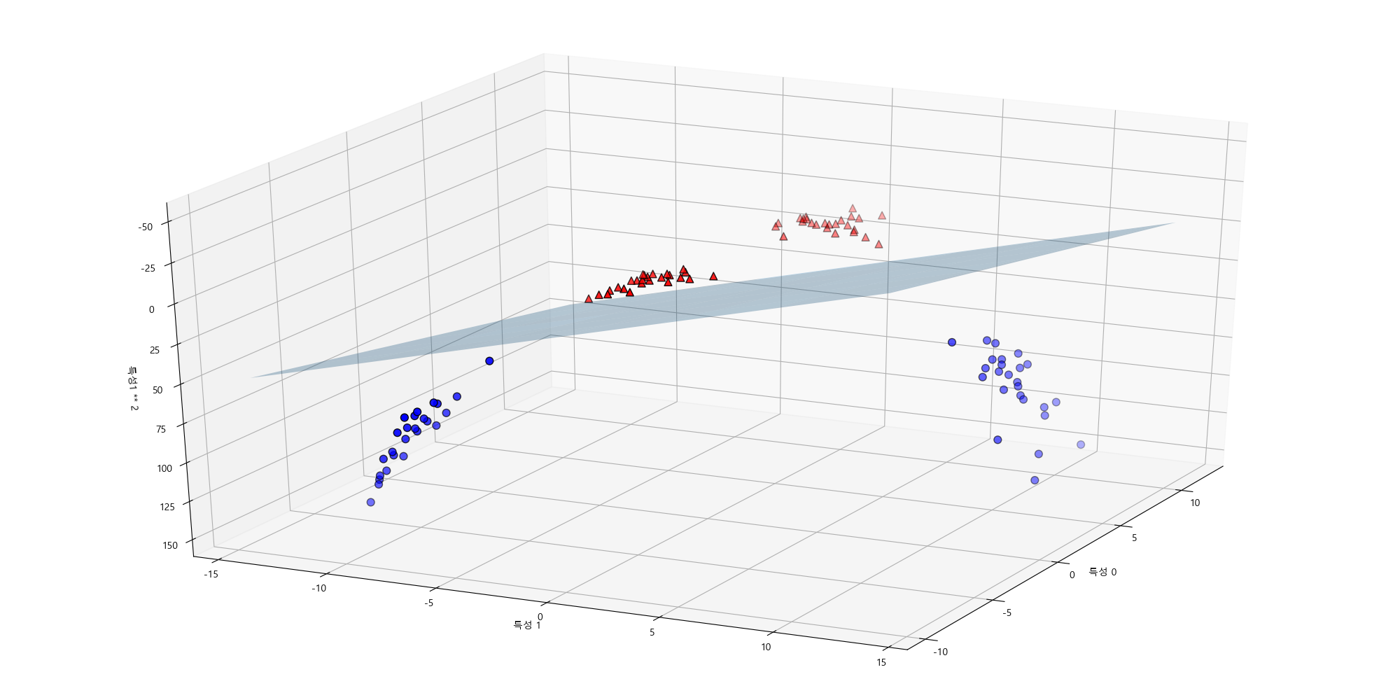
Example:
Imagine predicting whether a company will be profitable (1) or not (0) based on:
- Marketing Budget ($ x_1 $)
- R&D Investment ($ x_2 $)
- Number of Employees ($ x_3 $)
The decision boundary would be a plane in 3D space, separating profitable and non-profitable companies.
In general, for n features, the decision boundary is a hyperplane in an n-dimensional space.
4. Non-Linear Decision Boundaries in Depth
So far, we have seen that logistic regression creates linear decision boundaries. However, many real-world problems have non-linear relationships. In such cases, a straight line (or plane) is not sufficient to separate classes.
To capture complex decision boundaries, we introduce polynomial features or feature transformations.
Example 1: Circular Decision Boundary
If the data requires a circular boundary, we can use quadratic terms:
$$ \theta_0 + \theta_1 x_1^2 + \theta_2 x_2^2 = 0 $$
This represents a circle in 2D space.
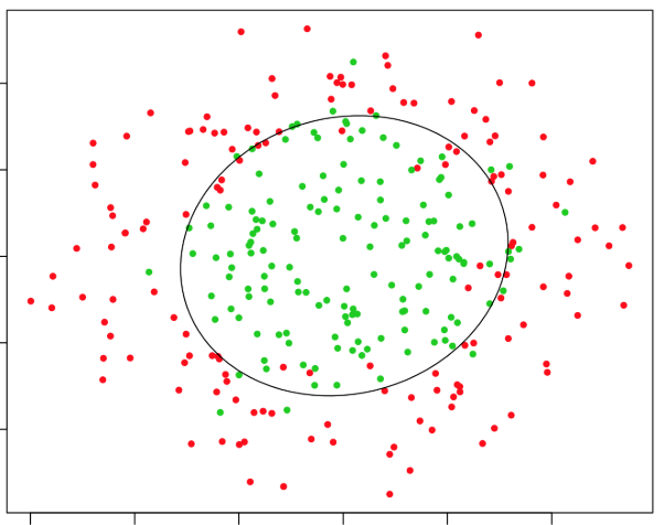
For example:
-
If $ x_1 $ and $ x_2 $ are the coordinates of points, a decision boundary like:
$$ x_1^2 + x_2^2 = 4 $$
would classify points inside a radius-2 circle as Class 1 and outside as Class 0.
Example 2: Elliptical Decision Boundary
A more general quadratic equation:
$$ \theta_0 + \theta_1 x_1^2 + \theta_2 x_2^2 + \theta_3 x_1 x_2 = 0 $$
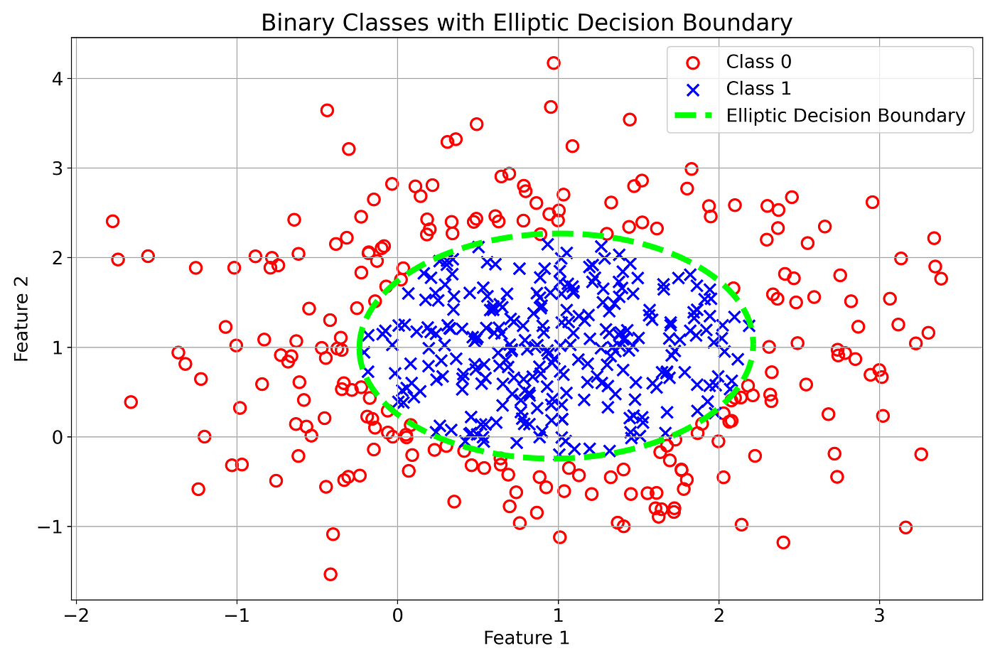
This allows for elliptical decision boundaries.
Example 3: Complex Non-Linear Boundaries
For even more complex boundaries, we can include higher-order polynomial features, such as:
$$ \theta_0 + \theta_1 x_1 + \theta_2 x_2 + \theta_3 x_1^2 + \theta_4 x_2^2 + \theta_5 x_1 x_2 + \theta_6 x_1^3 + \theta_7 x_2^3 = 0 $$
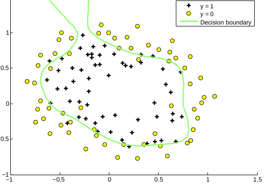
This enables twists and curves in the decision boundary, allowing logistic regression to model highly non-linear patterns.
Feature Engineering for Non-Linear Boundaries
- Instead of adding polynomial terms manually, we can transform features using basis functions (e.g., Gaussian kernels or radial basis functions).
- Feature maps can convert non-linearly separable data into a higher-dimensional space where a linear decision boundary works.
Limitations of Logistic Regression for Non-Linear Boundaries
- Feature engineering is required: Unlike neural networks or decision trees, logistic regression cannot learn complex boundaries automatically.
- Higher-degree polynomials can lead to overfitting: Too many non-linear terms make the model sensitive to noise.
Key Takeaways
- In 3D, the decision boundary is a plane, and in higher dimensions, it becomes a hyperplane.
- Non-linear decision boundaries can be created using quadratic, cubic, or transformed features.
- Feature engineering is crucial to make logistic regression work well for non-linearly separable problems.
- Too many high-order polynomial terms can cause overfitting, so regularization is needed.
3. Cost Function for Logistic Regression
1. Why Do We Need a Cost Function?
In linear regression, we use the Mean Squared Error (MSE) as the cost function:
$$ J(\theta) = \frac{1}{m} \sum_{i=1}^{m} (h_θ(x_i) - y_i)^2 $$
However, this cost function does not work well for logistic regression because:
- The hypothesis function in logistic regression is non-linear due to the sigmoid function.
- Using squared errors results in a non-convex function with multiple local minima, making optimization difficult.
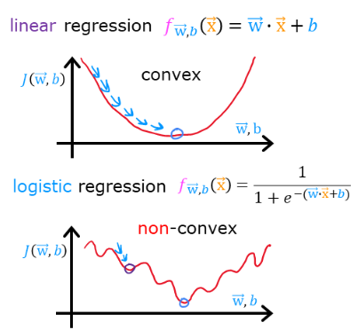
We need a different cost function that:
✅ Works well with the sigmoid function.
✅ Is convex, so gradient descent can efficiently minimize it.
2. Simplified Cost Function for Logistic Regression
Instead of using squared errors, we use a log loss function:
$$ J(\theta) = -\frac{1}{m} \sum_{i=1}^{m} \left[ y_i \log(h_θ(x_i)) + (1 - y_i) \log(1 - h_θ(x_i)) \right] $$
Where:
- $ y_i $ is the true label (0 or 1).
- $ h_θ(x_i) $ is the predicted probability from the sigmoid function.
This function ensures:
- If $ y = 1 $ → The first term dominates: $ -\log(h_θ(x)) $, which is close to 0 if $ h_\theta(x) \approx 1 $ (correct prediction).
- If $ y = 0 $ → The second term dominates: $ -\log(1 - h_θ(x)) $, which is close to 0 if $ h_\theta(x) \approx 0 $.
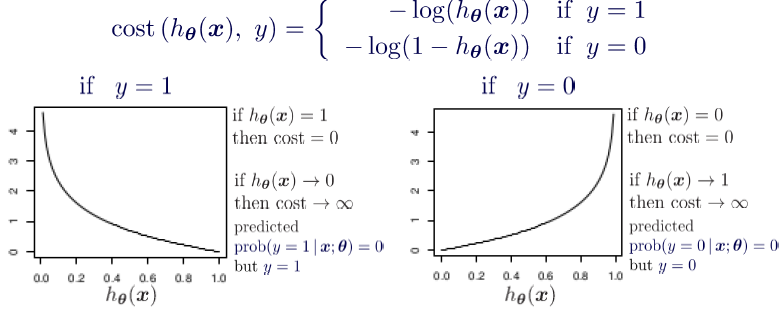
✅ Interpretation: The function penalizes incorrect predictions heavily while rewarding correct predictions.
3. Intuition Behind the Cost Function
Let’s break it down:
-
When $ y = 1 $, the cost function simplifies to:
$$ -\log(h_θ(x)) $$
This means:
- If $ h_θ(x) \approx 1 $ (correct prediction), $ -\log(1) = 0 $ → No penalty.
- If $ h_θ(x) \approx 0 $ (wrong prediction), $ -\log(0) \to \infty $ → High penalty!
-
When $ y = 0 $, the cost function simplifies to:
$$ -\log(1 - h_θ(x)) $$
This means:
- If $ h_θ(x) \approx 0 $ (correct prediction), $ -\log(1) = 0 $ → No penalty.
- If $ h_θ(x) \approx 1 $ (wrong prediction), $ -\log(0) \to \infty $ → High penalty!
✅ Key Takeaway:
The function assigns very high penalties for incorrect predictions, encouraging the model to learn correct classifications.
4. Gradient Descent for Logistic Regression
1. Why Do We Need Gradient Descent?
In logistic regression, our goal is to find the best parameters $ \theta $ that minimize the cost function:
$$ J(\theta) = -\frac{1}{m} \sum_{i=1}^{m} \left[ y_i \log(h_{\theta}(x_i)) + (1 - y_i) \log(1 - h_{\theta}(x_i)) \right] $$
Since there is no closed-form solution like in linear regression, we use gradient descent to iteratively update $ \theta $ until we reach the minimum cost.
2. Gradient Descent Algorithm
Gradient descent updates the parameters using the rule:
$$ \theta_j := \theta_j - \alpha \frac{\partial J(\theta)}{\partial \theta_j} $$
Where:
- $ \alpha $ is the learning rate (step size).
- $ \frac{\partial J(\theta)}{\partial \theta_j} $ is the gradient (direction of steepest increase).
For logistic regression, the derivative of the cost function is:
$$ \frac{\partial J(\theta)}{\partial \theta_j} = \frac{1}{m} \sum_{i=1}^{m} (h_{\theta}(x_i) - y_i) x_{ij} $$
Thus, the update rule becomes:
$$ \theta_j := \theta_j - \alpha \frac{1}{m} \sum_{i=1}^{m} (h_{\theta}(x_i) - y_i) x_{ij} $$
✅ Key Insight:
- We compute the error: $ h_θ(x_i) - y_i $.
- Multiply it by the feature $ x_{ij} $.
- Average over all training examples.
- Scale by $ \alpha $ and update $ \theta_j $.
Overfitting and Regularization
- 1. The Problem of Overfitting
- 2. Addressing Overfitting
- 3. Regularized Cost Function
- 4. Regularized Linear Regression
- 5. Regularized Logistic Regression
1. The Problem of Overfitting
What is Overfitting?
Overfitting occurs when a machine learning model learns the training data too well, capturing noise and random fluctuations rather than the underlying pattern. As a result, the model performs well on training data but generalizes poorly to unseen data.
Symptoms of Overfitting
- High training accuracy but low test accuracy (poor generalization).
- Complex decision boundaries that fit training data too closely.
- Large model parameters (high magnitude weights), leading to excessive sensitivity to small changes in input data.
Example of Overfitting in Regression
Consider a polynomial regression model. If we fit a high-degree polynomial to data, the model may pass through all training points perfectly but fail to predict new data correctly.
Overfitting vs. Underfitting
| Model Complexity | Training Error | Test Error | Generalization |
|---|---|---|---|
| Underfitting (High Bias) | High | High | Poor |
| Good Fit | Low | Low | Good |
| Overfitting (High Variance) | Very Low | High | Poor |
Visualization of Overfitting
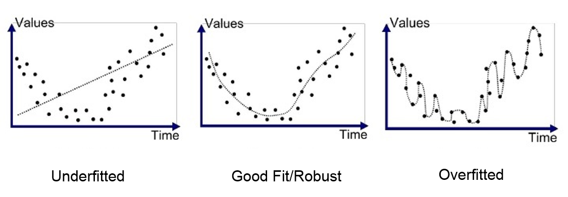
- Left (Underfitting): The model is too simple and cannot capture the trend.
- Middle (Good Fit): The model captures the pattern without overcomplicating.
- Right (Overfitting): The model follows the training data too closely, failing on new inputs.
2. Addressing Overfitting
Overfitting occurs when a model learns noise instead of the underlying pattern in the data. To address overfitting, we can apply several strategies to improve the model’s ability to generalize to unseen data.
1. Collecting More Data
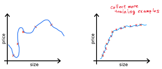
- More training data helps the model capture real patterns rather than memorizing noise.
- Especially effective for deep learning models, where small datasets tend to overfit quickly.
- Not always feasible, but can be supplemented with data augmentation techniques.
2. Feature Selection & Engineering
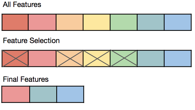
- Removing irrelevant or redundant features reduces model complexity.
- Techniques like Principal Component Analysis (PCA) help reduce dimensionality.
- Engineering new features (e.g., creating polynomial features or interaction terms) can improve generalization.
3. Cross-Validation
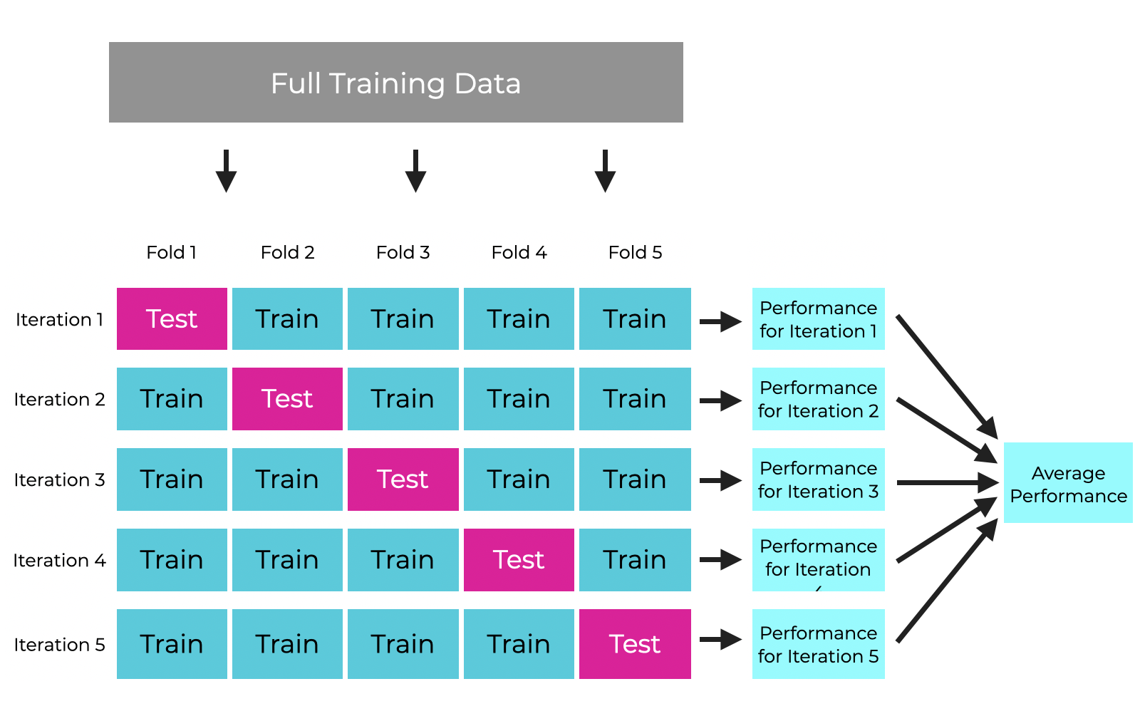
- k-fold cross-validation ensures that the model performs well on different data splits.
- Helps detect overfitting early by testing the model on multiple subsets of data.
- Leave-one-out cross-validation (LOOCV) is another approach, especially useful for small datasets.
4. Regularization as a Solution
- Regularization techniques add constraints to the model to prevent excessive complexity.
- L1 (Lasso) and L2 (Ridge) Regularization introduce penalties for large coefficients.
- We will explore regularized cost functions in the next section.
By applying these techniques, we control model complexity and improve generalization performance. In the next section, we will dive deeper into regularization and its role in the cost function.
3. Regularized Cost Function
Overfitting often occurs when a model learns excessive complexity, leading to poor generalization. One way to control this is by modifying the cost function to penalize overly complex models.
1. Why Modify the Cost Function?
The standard cost function in regression or classification only minimizes the error on training data, which can result in large coefficients (weights) that overfit the data.
By adding a regularization term, we discourage large weights, making the model simpler and reducing overfitting.
2. Adding Regularization Term
Regularization adds a penalty term to the cost function that shrinks the model parameters. The two most common types of regularization are:
L2 Regularization (Ridge Regression)
In L2 regularization, we add the sum of squared weights to the cost function:
$$ J(\theta) = \frac{1}{m} \sum_{i=1}^{m} \left[ h_\theta(x^{(i)}) - y^{(i)} \right]^2 + \lambda \sum_{j=1}^{n} \theta_j^2 $$
- $\lambda$ (regularization parameter) controls how much regularization is applied.
- Higher $\lambda$ values force the model to reduce the magnitude of parameters, preventing overfitting.
- L2 regularization keeps all features but reduces their impact.
L1 Regularization (Lasso Regression)
In L1 regularization, we add the absolute values of weights:
$$ J(\theta) = \frac{1}{m} \sum_{i=1}^{m} \left[ h_\theta(x^{(i)}) - y^{(i)} \right]^2 + \lambda \sum_{j=1}^{n} |\theta_j| $$
- L1 regularization pushes some coefficients to zero, effectively performing feature selection.
- It results in sparser models, which are useful when many features are irrelevant.
3. Effect of Regularization on Model Complexity
Regularization controls model complexity by restricting parameter values:
- No Regularization ($\lambda = 0$) → The model fits the training data too closely (overfitting).
- Small $\lambda$ → The model is still flexible but generalizes better.
- Large $\lambda$ → The model becomes too simple (underfitting), losing important patterns.
Visualization of Regularization Effects
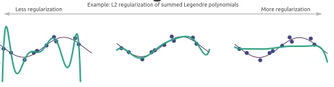
- Left (No Regularization): The model overfits training data.
- Middle (Moderate Regularization): The model generalizes well.
- Right (Strong Regularization): The model underfits the data.
4. Regularized Linear Regression
Linear regression without regularization can suffer from overfitting, especially when the model has too many features or when training data is limited. Regularization helps by constraining the model’s parameters, preventing extreme values that lead to high variance.
1. Linear Regression Cost Function (Without Regularization)
The standard cost function for linear regression is:
$$ J(\theta) = \frac{1}{2m} \sum_{i=1}^{m} \left( h_\theta(x^{(i)}) - y^{(i)} \right)^2 $$
where:
- $ h_\theta(x) = \theta^T x $ is the hypothesis (predicted value),
- $ m $ is the number of training examples.
This function minimizes the sum of squared errors but does not impose any restrictions on the parameter values, which can lead to overfitting.
2. Regularized Cost Function for Linear Regression
To prevent overfitting, we add an L2 regularization term (also known as Ridge Regression) to penalize large parameter values:
$$ J(\theta) = \frac{1}{2m} \sum_{i=1}^{m} \left( h_\theta(x^{(i)}) - y^{(i)} \right)^2 + \frac{\lambda}{2m} \sum_{j=1}^{n} \theta_j^2 $$
where:
- $ \lambda $ is the regularization parameter that controls the penalty,
- The term $ \sum \theta_j^2 $ penalizes large values of $ \theta $,
- $ \theta_0 $ (bias term) is not regularized.
3. Effect of Regularization in Gradient Descent
Regularization modifies the gradient descent update rule:
$$ \theta_j := \theta_j - \alpha \left[ \frac{1}{m} \sum_{i=1}^{m} \left( h_\theta(x^{(i)}) - y^{(i)} \right) x_j + \frac{\lambda}{m} \theta_j \right] $$
- The additional term $ \frac{\lambda}{m} \theta_j $ shrinks the parameter values over time.
- When $ \lambda $ is too large, the model underfits (too simple).
- When $ \lambda $ is too small, the model overfits (too complex).
Effect of Regularization on Parameters
- If $ \lambda = 0 $: Regularization is off → Overfitting risk.
- If $ \lambda $ is too high: Model is too simple → Underfitting.
- If $ \lambda $ is optimal: Good generalization → Balanced model.
4. Normal Equation with Regularization
For linear regression, we can solve for $ \theta $ using the Normal Equation, which avoids gradient descent:
$$ \theta = (X^T X + \lambda I)^{-1} X^T y $$
where:
- $ I $ is the identity matrix (except $ \theta_0 $ is not regularized).
- Adding $ \lambda I $ ensures $ X^T X $ is invertible, reducing multicollinearity issues.
5. Summary
✅ Regularization reduces overfitting by penalizing large weights.
✅ L2 regularization (Ridge Regression) modifies cost function by adding $ \sum \theta_j^2 $.
✅ Gradient Descent and Normal Equation both adjust to include regularization.
✅ Choosing $ \lambda $ is critical: too high → underfitting, too low → overfitting.
5. Regularized Logistic Regression
Logistic regression is commonly used for classification tasks, but like linear regression, it can overfit when there are too many features or limited data. Regularization helps control overfitting by penalizing large parameter values.
1. Logistic Regression Cost Function (Without Regularization)
The standard cost function for logistic regression is:
$$ J(\theta) = -\frac{1}{m} \sum_{i=1}^{m} \left[ y^{(i)} \log h_\theta(x^{(i)}) + (1 - y^{(i)}) \log (1 - h_\theta(x^{(i)})) \right] $$
where:
- $ h_\theta(x) = \frac{1}{1 + e^{-\theta^T x}} $ is the sigmoid function,
- $ y $ is the actual class label ($ 0 $ or $ 1 $),
- $ m $ is the number of training examples.
This cost function does not include regularization, meaning the model may assign large weights to some features, leading to overfitting.
2. Regularized Cost Function for Logistic Regression
To reduce overfitting, we add an L2 regularization term, similar to regularized linear regression:
$$ J(\theta) = -\frac{1}{m} \sum_{i=1}^{m} \left[ y^{(i)} \log h_\theta(x^{(i)}) + (1 - y^{(i)}) \log (1 - h_\theta(x^{(i)})) \right] + \frac{\lambda}{2m} \sum_{j=1}^{n} \theta_j^2 $$
where:
- $ \lambda $ is the regularization parameter (controls penalty),
- The term $ \sum \theta_j^2 $ discourages large parameter values,
- $ \theta_0 $ (bias term) is NOT regularized.
✅ Effect of Regularization
- Small $ \lambda $ → Model may overfit (complex decision boundary).
- Large $ \lambda $ → Model may underfit (too simple, missing important features).
- Optimal $ \lambda $ → Model generalizes well.
3. Effect of Regularization in Gradient Descent
Regularization modifies the gradient descent update rule:
$$ \theta_j := \theta_j - \alpha \left[ \frac{1}{m} \sum_{i=1}^{m} \left( h_\theta(x^{(i)}) - y^{(i)} \right) x_j + \frac{\lambda}{m} \theta_j \right] $$
- The regularization term $ \frac{\lambda}{m} \theta_j $ shrinks the weight values over time.
- Helps avoid models that memorize training data instead of learning patterns.
4. Decision Boundary and Regularization
Regularization also affects decision boundaries:
- Without regularization ($ \lambda = 0 $): Complex boundaries that fit noise.
- With moderate $ \lambda $: Simpler boundaries that generalize better.
- With very high $ \lambda $: Too simplistic boundaries that underfit.
5. Summary
✅ Regularization in logistic regression prevents overfitting by controlling parameter sizes.
✅ L2 regularization (Ridge Regression) adds $ \sum \theta_j^2 $ to cost function.
✅ Gradient Descent is adjusted to shrink large weights.
✅ Choosing $ \lambda $ is critical for a well-generalized model.
Scikit-learn: Practical Applications
- 1. Introduction to Scikit-Learn
- 2. Linear Regression with Scikit-Learn
- 3. Multiple Linear Regression with Scikit-Learn
- 4. Polynomial Regression with Scikit-Learn
- 5. Binary Classification with Logistic Regression
- 6. Multi-Class Classification with Logistic Regression
1. Introduction to Scikit-Learn
Scikit-Learn is one of the most popular and powerful Python libraries for machine learning. It provides efficient implementations of various machine learning algorithms and tools for data preprocessing, model selection, and evaluation. It is built on top of NumPy, SciPy, and Matplotlib, making it highly compatible with the scientific computing ecosystem in Python.
Why Use Scikit-Learn?
- Easy to Use: Provides a simple and consistent API for machine learning models.
- Comprehensive: Includes a wide range of algorithms, including regression, classification, clustering, and dimensionality reduction.
- Efficient: Implements fast and optimized versions of ML algorithms.
- Integration: Works well with other libraries like Pandas, NumPy, and Matplotlib.
Loading Built-in Datasets in Scikit-Learn
Scikit-Learn provides several built-in datasets that can be used for practice and experimentation. Some common datasets include:
- Iris Dataset (
load_iris): Classification dataset for flower species. - Boston Housing Dataset (
load_boston) (Deprecated): Regression dataset for predicting house prices. - Digits Dataset (
load_digits): Handwritten digit classification. - Wine Dataset (
load_wine): Classification dataset for different types of wine. - Breast Cancer Dataset (
load_breast_cancer): Binary classification dataset for cancer diagnosis.
Example: Loading and Exploring the Iris Dataset
from sklearn.datasets import load_iris
import pandas as pd

# Load the dataset
iris = load_iris()

# Convert to DataFrame
iris_df = pd.DataFrame(iris.data, columns=iris.feature_names)

# Add target labels
iris_df['target'] = iris.target

# Display first few rows
print(iris_df.head())
Splitting Data: Train-Test Split
To evaluate a machine learning model, we need to split the data into a training set and a test set. This ensures that we can measure the model’s performance on unseen data.
Scikit-Learn provides train_test_split for this purpose:
Example: Splitting the Iris Dataset
from sklearn.model_selection import train_test_split

# Features and target variable
X = iris.data
y = iris.target

# Split into 80% training and 20% testing
X_train, X_test, y_train, y_test = train_test_split(X, y, test_size=0.2, random_state=42)

print(f"Training samples: {len(X_train)}, Testing samples: {len(X_test)}")
test_size=0.2means 20% of the data is reserved for testing.random_state=42ensures reproducibility.
By following these steps, we have successfully loaded a dataset and prepared it for machine learning. In the next section, we will explore how to apply Linear Regression using Scikit-Learn.
Train-Test Split and Why It Matters
When training a machine learning model, we must evaluate its performance on unseen data to ensure it generalizes well. This is done by splitting the dataset into training and test sets.
Why Not Use 100% of Data for Training?
If we train the model using all available data, we won’t have any independent data to check how well it performs on new inputs. This leads to overfitting, where the model memorizes the training data instead of learning general patterns.
Why Not Use 90% or More for Testing?
While a large test set gives a better estimate of real-world performance, it reduces the amount of data available for training. A model trained on very little data may suffer from underfitting—it won’t have enough information to learn meaningful patterns.
What’s the Ideal Train-Test Split?
A commonly used ratio is 80% for training, 20% for testing. However, this depends on:
- Dataset Size: If data is limited, we may use a 90/10 split to keep more training data.
- Model Complexity: Simpler models may work with less training data, but deep learning models require more.
- Use Case: In critical applications (e.g., medical diagnosis), a larger test set (e.g., 30%) is preferred for reliable evaluation.
Key Takeaways
✅ 80/20 is a good starting point, but can vary based on dataset size and model needs.
✅ Too small a test set → Unreliable performance evaluation.
✅ Too large a test set → Model may not have enough training data to learn properly.
✅ Always shuffle the data before splitting to avoid biased results.
2. Linear Regression with Scikit-Learn
1. Introduction to Linear Regression
Linear regression is a fundamental supervised learning algorithm used to model the relationship between a dependent variable (target) and one or more independent variables (features). It assumes a linear relationship between input features and the output.
The mathematical form of a simple linear regression model is:
$$ y = \theta_0 + \theta_1 x $$
Where:
- $y$ is the predicted output.
- $x$ is the input feature.
- $\theta_0$ is the intercept (bias).
- $\theta_1$ is the coefficient (weight) of the feature.
Now, let’s implement a simple linear regression model using Scikit-Learn.
2. Importing Required Libraries
First, we import necessary libraries for handling data, building the model, and evaluating its performance.
import numpy as np
import matplotlib.pyplot as plt
import pandas as pd
from sklearn.model_selection import train_test_split
from sklearn.linear_model import LinearRegression
from sklearn.metrics import mean_squared_error, r2_score
3. Creating a Sample Dataset
We will generate a synthetic dataset to train and test our linear regression model.
# Generate random data
np.random.seed(42)  # Ensures reproducibility
X = 2 * np.random.rand(100, 1)  # 100 samples, single feature
y = 4 + 3 * X + np.random.randn(100, 1)  # y = 4 + 3X + Gaussian noise

# Convert to a DataFrame for better visualization
df = pd.DataFrame(np.hstack((X, y)), columns=["Feature X", "Target y"])
df.head()
np.random.rand(100, 1): Generates $100$ random values between $0$ and $2$.y = 4 + 3X + noise: Defines a linear relationship with some added noise.- We use
pd.DataFrameto display the first few samples.
4. Splitting Data into Training and Testing Sets
It is crucial to split the dataset into training and testing sets to evaluate model performance on unseen data.
# Splitting dataset into 80% training and 20% testing
X_train, X_test, y_train, y_test = train_test_split(X, y, test_size=0.2, random_state=42)

print(f"Training set size: {X_train.shape[0]} samples")
print(f"Testing set size: {X_test.shape[0]} samples")
5. Training the Linear Regression Model
Now, we train a linear regression model using Scikit-Learn’s LinearRegression() class.
# Create and train the model
model = LinearRegression()
model.fit(X_train, y_train)

# Print learned parameters
print(f"Intercept (theta_0): {model.intercept_[0]:.2f}")
print(f"Coefficient (theta_1): {model.coef_[0][0]:.2f}")
fit(X_train, y_train): Trains the model by finding the best-fitting line.model.intercept_: The learned bias term.model.coef_: The learned weight for the feature.
6. Making Predictions
After training, we make predictions on the test set.
# Predict on test data
y_pred = model.predict(X_test)

# Compare actual vs predicted values
comparison_df = pd.DataFrame({"Actual": y_test.flatten(), "Predicted": y_pred.flatten()})
comparison_df.head()
model.predict(X_test): Generates predictions.- The DataFrame compares actual vs. predicted values.
7. Evaluating the Model
We use Mean Squared Error (MSE) and R² Score to evaluate model performance.
# Calculate Mean Squared Error (MSE)
mse = mean_squared_error(y_test, y_pred)

# Calculate R-squared score
r2 = r2_score(y_test, y_pred)

print(f"Mean Squared Error: {mse:.2f}")
print(f"R-squared Score: {r2:.2f}")
- MSE: Measures average squared differences between actual and predicted values (lower is better).
- R² Score: Measures how well the model explains the variance in the data (closer to 1 is better).
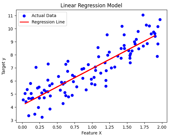
8. Visualizing the Results
Finally, let’s plot the data and the regression line.
plt.scatter(X, y, color="blue", label="Actual Data")
plt.plot(X_test, y_pred, color="red", linewidth=2, label="Regression Line")
plt.xlabel("Feature X")
plt.ylabel("Target y")
plt.title("Linear Regression Model")
plt.legend()
plt.show()
This plot shows:
- Blue points → Actual test data
- Red line → Best-fit regression line
3. Multiple Linear Regression with Scikit-Learn
What is Multiple Linear Regression?
Multiple Linear Regression is an extension of simple linear regression where we predict a dependent variable ($y$) using multiple independent variables ($x_1, x_2, …, x_n$). The general form of the equation is:
$$ y = \theta_0 + \theta_1 x_1 + \theta_2 x_2 + … + \theta_n x_n $$
Where:
- $ y $ = predicted output
- $ x_1, x_2, …, x_n $ = independent variables (features)
- $ \theta_0 $ = intercept
- $ \theta_1, \theta_2, …, \theta_n $ = coefficients (weights)
In this section, we will:
- Generate a synthetic dataset for a multiple linear regression model.
- Train a model using Scikit-Learn.
- Visualize the relationship in a 3D plot.
Step 1: Generate a Synthetic Dataset
First, let’s create a dataset with two independent variables ($x_1$ and $x_2$) and one dependent variable ($y$). We’ll add some noise to make it more realistic.
import numpy as np
import matplotlib.pyplot as plt
from mpl_toolkits.mplot3d import Axes3D
from sklearn.linear_model import LinearRegression
from sklearn.model_selection import train_test_split

# Set seed for reproducibility
np.random.seed(42)

# Generate random data for x1 and x2
x1 = np.random.uniform(0, 10, 100)
x2 = np.random.uniform(0, 10, 100)

# Define the true equation y = 3 + 2*x1 + 1.5*x2 + noise
y = 3 + 2*x1 + 1.5*x2 + np.random.normal(0, 2, 100)

# Reshape x1 and x2 for model training
X = np.column_stack((x1, x2))
Step 2: Train the Model
Now, we split the dataset into training and test sets and train a multiple linear regression model.
# Split data into training and test sets
X_train, X_test, y_train, y_test = train_test_split(X, y, test_size=0.2, random_state=42)

# Create and train the model
model = LinearRegression()
model.fit(X_train, y_train)

# Get model parameters
theta0 = model.intercept_
theta1, theta2 = model.coef_
print(f"Model equation: y = {theta0:.2f} + {theta1:.2f}*x1 + {theta2:.2f}*x2")
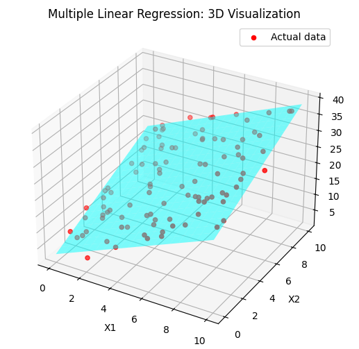
Step 3: Visualize the Regression Plane
Since we have two independent variables ($x_1$ and $x_2$), we can plot the regression plane in 3D space.
# Generate grid for x1 and x2
x1_range = np.linspace(0, 10, 20)
x2_range = np.linspace(0, 10, 20)
x1_grid, x2_grid = np.meshgrid(x1_range, x2_range)

# Compute predicted y values
y_pred_grid = theta0 + theta1 * x1_grid + theta2 * x2_grid

# Create 3D plot
fig = plt.figure(figsize=(10, 6))
ax = fig.add_subplot(111, projection='3d')

# Scatter plot of real data
ax.scatter(x1, x2, y, color='red', label='Actual data')

# Regression plane
ax.plot_surface(x1_grid, x2_grid, y_pred_grid, alpha=0.5, color='cyan')

# Labels
ax.set_xlabel('X1')
ax.set_ylabel('X2')
ax.set_zlabel('Y')
ax.set_title('Multiple Linear Regression: 3D Visualization')
plt.legend()
plt.show()
Key Takeaways
- We generated a dataset with two independent variables and one dependent variable.
- We trained a Multiple Linear Regression model using Scikit-Learn.
- We visualized the regression plane in 3D, showing how $x_1$ and $x_2$ influence $y$.
4. Polynomial Regression with Scikit-Learn
Polynomial Regression is an extension of Linear Regression, where we introduce polynomial terms to capture non-linear relationships in the data.
1. What is Polynomial Regression?
Linear regression models relationships using a straight line:
$$ y = \theta_0 + \theta_1 x $$
However, if the data follows a non-linear pattern, a straight line won’t fit well. Instead, we can introduce polynomial terms:
$$ y = \theta_0 + \theta_1 x + \theta_2 x^2 + \theta_3 x^3 + \dots + \theta_n x^n $$
This allows the model to capture curvature in the data.
2. Generating Non-Linear Data
First, let’s create a synthetic dataset with a non-linear relationship.
import numpy as np
import matplotlib.pyplot as plt

# Generate random x values between -3 and 3
np.random.seed(42)
X = np.linspace(-3, 3, 100).reshape(-1, 1)

# Generate a non-linear function with some noise
y = 0.5 * X**3 - X**2 + 2 + np.random.randn(100, 1) * 2

# Scatter plot of the data
plt.scatter(X, y, color='blue', alpha=0.5, label="True Data")
plt.xlabel("X")
plt.ylabel("y")
plt.title("Generated Non-Linear Data")
plt.legend()
plt.show()
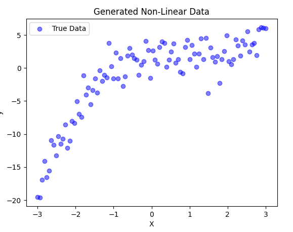
- We create 100 random points between -3 and 3.
- The function we generate follows a cubic equation:
- $y=0.5x^3 −x^2 +2$ with added noise.
- We visualize the data using a scatter plot.
3. Applying Polynomial Features
To transform our linear features into polynomial features, we use PolynomialFeatures from sklearn.preprocessing.
from sklearn.preprocessing import PolynomialFeatures

# Transform X into polynomial features (degree=3)
poly = PolynomialFeatures(degree=3)
X_poly = poly.fit_transform(X)

print(f"Original X shape: {X.shape}")
print(f"Transformed X shape: {X_poly.shape}")
print(f"First 5 rows of X_poly:\n{X_poly[:5]}")
- We use
PolynomialFeatures(degree=3)to add polynomial terms up to $x^3$. - This converts each $𝑥$ value into a feature vector $[1,x,x^2,x^3]$.
- We print the new shape and first few transformed rows.
4. Training a Polynomial Regression Model
Now, we train a Linear Regression model using these polynomial features.
from sklearn.linear_model import LinearRegression

# Train polynomial regression model
model = LinearRegression()
model.fit(X_poly, y)

# Predictions
y_pred = model.predict(X_poly)
5. Visualizing the Results
Let’s plot the polynomial regression model against the actual data.
plt.scatter(X, y, color='blue', alpha=0.5, label="True Data")
plt.plot(X, y_pred, color='red', linewidth=2, label="Polynomial Regression Fit")
plt.xlabel("X")
plt.ylabel("y")
plt.title("Polynomial Regression Model")
plt.legend()
plt.show()
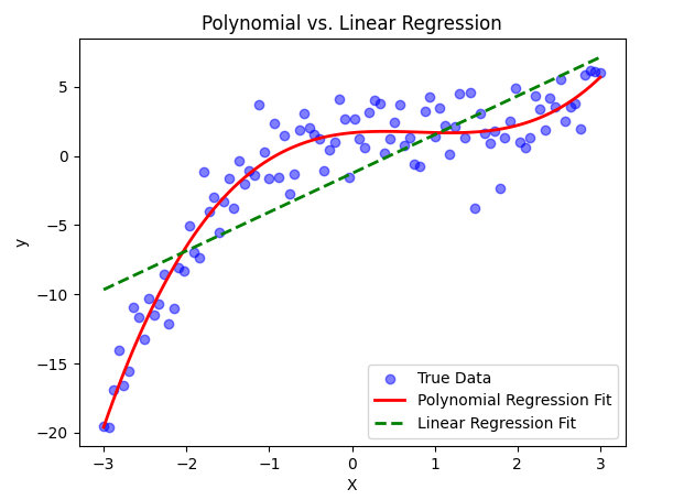
6. Comparing with Linear Regression
Now, let’s compare Polynomial Regression with a simple Linear Regression model.
# Train a simple Linear Regression model
linear_model = LinearRegression()
linear_model.fit(X, y)
y_linear_pred = linear_model.predict(X)

# Plot both models
plt.scatter(X, y, color='blue', alpha=0.5, label="True Data")
plt.plot(X, y_pred, color='red', linewidth=2, label="Polynomial Regression Fit")
plt.plot(X, y_linear_pred, color='green', linestyle="dashed", linewidth=2, label="Linear Regression Fit")
plt.xlabel("X")
plt.ylabel("y")
plt.title("Polynomial vs. Linear Regression")
plt.legend()
plt.show()
5. Binary Classification with Logistic Regression
Logistic Regression is a fundamental algorithm used for binary classification problems. It estimates the probability that a given input belongs to a particular class using the sigmoid function.
1. What is Logistic Regression?
Unlike Linear Regression, which predicts continuous values, Logistic Regression predicts probabilities and then maps them to class labels (0 or 1). The model is defined as:
$$ P(y=1 | X) = \frac{1}{1 + e^{-\theta^T X}} $$
Where:
- $\theta$ represents the model parameters (weights and bias).
- $X$ represents the input features.
- The output is a probability between 0 and 1.
2. Generating a Synthetic Dataset (Spam Detection Example)
We’ll create a synthetic dataset where emails are classified as spam (1) or not spam (0) based on two features:
- Number of suspicious words
- Email length
import numpy as np
import matplotlib.pyplot as plt
from sklearn.model_selection import train_test_split
from sklearn.linear_model import LogisticRegression
from sklearn.metrics import accuracy_score

# Generating synthetic data
np.random.seed(42)
num_samples = 200

# Feature 1: Number of suspicious words (randomly chosen values)
suspicious_words = np.random.randint(0, 20, num_samples)

# Feature 2: Email length (short emails tend to be spammy)
email_length = np.random.randint(20, 300, num_samples)

# Labels: Spam (1) or Not Spam (0)
labels = (suspicious_words + email_length / 50 > 10).astype(int)

# Creating feature matrix
X = np.column_stack((suspicious_words, email_length))
y = labels

# Splitting into training and testing sets
X_train, X_test, y_train, y_test = train_test_split(X, y, test_size=0.2, random_state=42)
3. Training the Logistic Regression Model
Now, we train a Logistic Regression model on our dataset.
# Training the model
model = LogisticRegression()
model.fit(X_train, y_train)

# Making predictions
y_pred = model.predict(X_test)

# Evaluating the model
accuracy = accuracy_score(y_test, y_pred)
print(f"Model Accuracy: {accuracy:.2f}")
4. Visualizing Decision Boundary
The decision boundary helps us see how the model separates spam from non-spam emails. We plot the boundary in 2D.
# Function to plot decision boundary
def plot_decision_boundary(model, X, y):
    x_min, x_max = X[:, 0].min() - 1, X[:, 0].max() + 1
    y_min, y_max = X[:, 1].min() - 10, X[:, 1].max() + 10
    xx, yy = np.meshgrid(np.linspace(x_min, x_max, 100),
                         np.linspace(y_min, y_max, 100))

    Z = model.predict(np.c_[xx.ravel(), yy.ravel()])
    Z = Z.reshape(xx.shape)

    plt.contourf(xx, yy, Z, alpha=0.3, cmap=plt.cm.coolwarm)
    plt.scatter(X[:, 0], X[:, 1], c=y, edgecolors='k', cmap=plt.cm.coolwarm)
    plt.xlabel("Suspicious Words Count")
    plt.ylabel("Email Length")
    plt.title("Logistic Regression Decision Boundary")
    plt.show()

# Plotting the decision boundary
plot_decision_boundary(model, X, y)
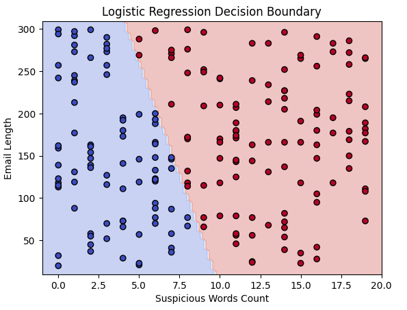
This plot shows how the model separates spam and non-spam emails using our two features.
Key Takeaways
- Logistic Regression is used for binary classification.
- It estimates probabilities using the sigmoid function.
- We generated a synthetic dataset mimicking spam detection.
- We trained and evaluated a Logistic Regression model.
- Decision boundaries help visualize how the model classifies data.
6. Multi-Class Classification with Logistic Regression
In this section, we will implement a Multi-Class Classification model using Logistic Regression. Instead of a binary classification problem, we will classify data points into three distinct categories.
This project predicts a student’s success level based on study hours and past grades using Logistic Regression.
We classify students into three categories:
- Fail (0)
- Pass (1)
- High Pass (2)
Step 1: Import Libraries
We start by importing necessary libraries for:
- Data generation
- Visualization
- Model training
import numpy as np
import matplotlib.pyplot as plt
from sklearn.datasets import make_classification
from sklearn.model_selection import train_test_split
from sklearn.preprocessing import StandardScaler
from sklearn.linear_model import LogisticRegression
from sklearn.metrics import ConfusionMatrixDisplay, classification_report
Step 2: Generate Synthetic Data
We create artificial student data using make_classification.
Each student has:
- Past Grades (0-100)
- Study Hours (non-negative)
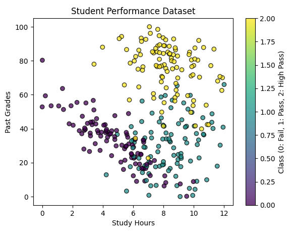
We set random_state = 457897 to ensure reproducibility.
# Generate a classification dataset
X, y = make_classification(n_samples=300,
                           n_features=2,
                           n_classes=3,
                           n_clusters_per_class=1,
                           n_informative=2,
                           n_redundant=0,
                           random_state=457897)  # Ensures consistent results

# Normalize Study Hours to be non-negative & scale Past Grades (0-100)
X[:, 0] = X[:, 0] * 12
X[:, 1] = X[:, 1] * 100

# Scatter plot of generated data
plt.figure(figsize=(7, 5))
plt.scatter(X[:, 0], X[:, 1], c=y, cmap='viridis', edgecolors='k', alpha=0.75)
plt.xlabel("Study Hours")
plt.ylabel("Past Grades")
plt.title("Student Performance Dataset")
plt.colorbar(label="Class (0: Fail, 1: Pass, 2: High Pass)")
plt.show()
Step 3: Split the Data
X_train, X_test, y_train, y_test = train_test_split(X, y, test_size=0.2, random_state=457897, stratify=y)

# Standardizing features for better model performance
scaler = StandardScaler()
X_train = scaler.fit_transform(X_train)
X_test = scaler.transform(X_test)
Step 4: Train Logistic Regression Model
from sklearn.multiclass import OneVsRestClassifier

# Define and train the model
model = OneVsRestClassifier(LogisticRegression(solver='lbfgs'))
model.fit(X_train, y_train)
Step 5: Visualizing Decision Boundaries
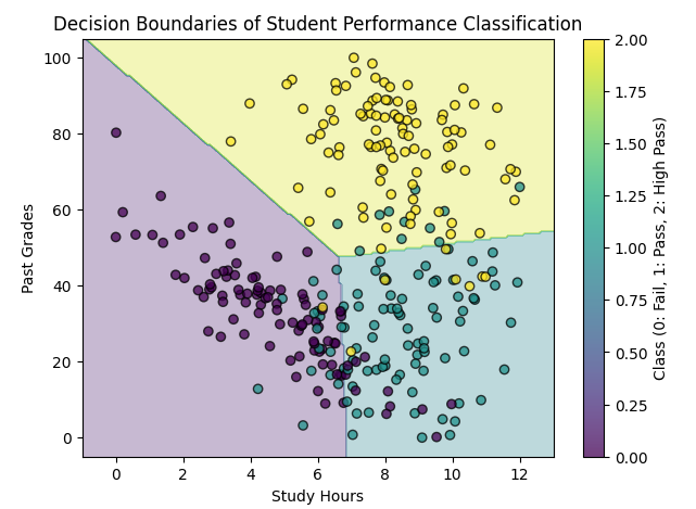
# Define a mesh grid for visualization
x_min, x_max = X[:, 0].min() - 1, X[:, 0].max() + 1
y_min, y_max = X[:, 1].min() - 5, X[:, 1].max() + 5
xx, yy = np.meshgrid(np.linspace(x_min, x_max, 200),
                     np.linspace(y_min, y_max, 200))

# Predict on the mesh grid
Z = model.predict(scaler.transform(np.c_[xx.ravel(), yy.ravel()]))
Z = Z.reshape(xx.shape)

# Plot decision boundary
plt.figure(figsize=(7, 5))
plt.contourf(xx, yy, Z, alpha=0.3, cmap="viridis")
plt.scatter(X[:, 0], X[:, 1], c=y, cmap="viridis", edgecolors='k', alpha=0.75)
plt.xlabel("Study Hours")
plt.ylabel("Past Grades")
plt.title("Decision Boundaries of Student Performance Classification")
plt.colorbar(label="Class (0: Fail, 1: Pass, 2: High Pass)")
plt.show()
Neural Networks: Intuition and Model
- Understanding Neural Networks
- Biological Inspiration: The Brain and Synapses
- Importance of Layers in Neural Networks
- Face Recognition Example: Layer-by-Layer Processing
- Mathematical Representation of a Neural Network
Understanding Neural Networks
Neural networks are a fundamental concept in deep learning, inspired by the way the human brain processes information. They consist of layers of artificial neurons that transform input data into meaningful outputs. At the core of a neural network is a simple mathematical operation: each neuron receives inputs, applies a weighted sum, adds a bias term, and passes the result through an activation function. This process allows the network to learn patterns and make predictions.
Biological Inspiration: The Brain and Synapses
Artificial neural networks (ANNs) are designed based on the biological structure of the human brain. The brain consists of billions of neurons, interconnected through structures called synapses. Neurons communicate with each other by transmitting electrical and chemical signals, which play a critical role in learning, memory, and decision-making processes.
Structure of a Biological Neuron
Each biological neuron consists of several key components:
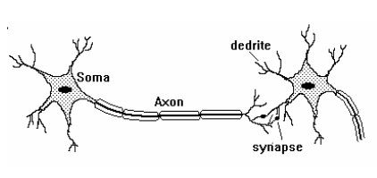
- Dendrites: Receive input signals from other neurons.
- Cell Body (Soma): Processes the received signals and determines whether the neuron should be activated.
- Axon: Transmits the output signal to other neurons.
- Synapses: Junctions between neurons where chemical neurotransmitters facilitate communication.
Artificial Neural Networks vs. Biological Networks
In artificial neural networks:
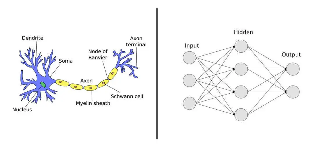
- Neurons function as computational units.
- Weights correspond to synaptic strengths, determining how influential an input is.
- Bias terms help shift the activation threshold.
- Activation functions mimic the way biological neurons fire only when certain thresholds are exceeded.
Importance of Layers in Neural Networks
Neural networks are composed of multiple layers, each responsible for extracting and processing features from input data. The more layers a network has, the deeper it becomes, allowing it to learn complex hierarchical patterns.
Example: Predicting a T-shirt’s Top-Seller Status
Consider an online clothing store that wants to predict whether a new T-shirt will become a top-seller. Several factors influence this outcome, which serve as inputs to our neural network:
- Price ($x_1$)
- Shipping Cost ($x_2$)
- Marketing ($x_3$)
- Material ($x_4$)
These inputs are fed into the first layer of the network, which extracts meaningful features. A possible hidden layer structure could be:
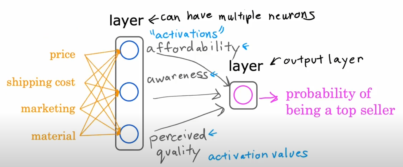
- Hidden Layer 1: Contains a few activations functions like: affordability , awareness, perceived quality.
- Output Layer: Aggregates information from the previous layers to make a final prediction.
The output layer applies a sigmoid activation function:
$$ \sigma(z) = \frac{1}{1 + e^{-z}} $$
where $z$ is a weighted sum of the previous layer’s outputs. If $\sigma(z) > 0.5$, we classify the T-shirt as a top-seller; otherwise, it is not.
Face Recognition Example: Layer-by-Layer Processing
Face recognition is a real-world example where neural networks excel. Let’s consider a deep neural network designed for face recognition, breaking down the processing step by step:
- Input Layer: An image of a face is converted into pixel values (e.g., a 100x100 grayscale image would be represented as a vector of 10,000 pixel values).
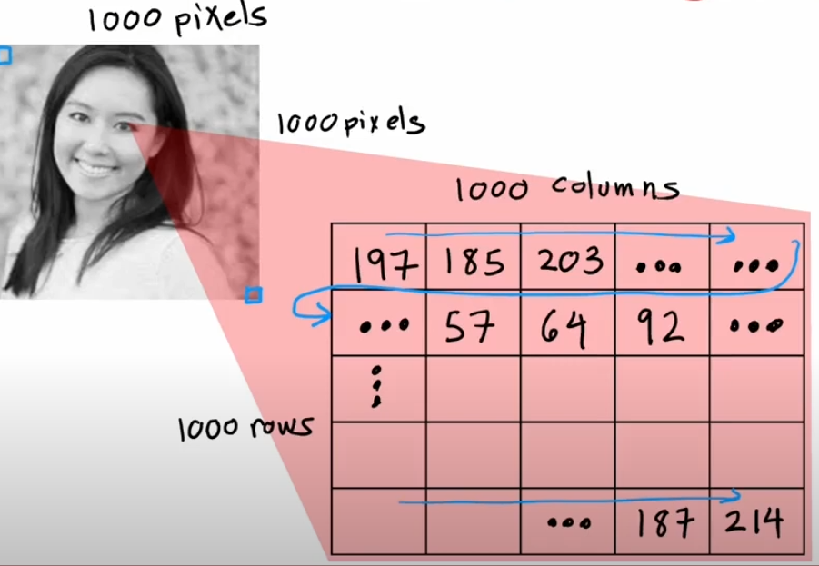
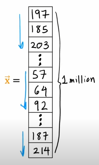
- First Hidden Layer: Detects basic edges and corners in the image by applying simple filters.
- Second Hidden Layer: Identifies facial features like eyes, noses, and mouths by combining edge and corner information.
- Third Hidden Layer: Recognizes entire facial structures and relationships between features.
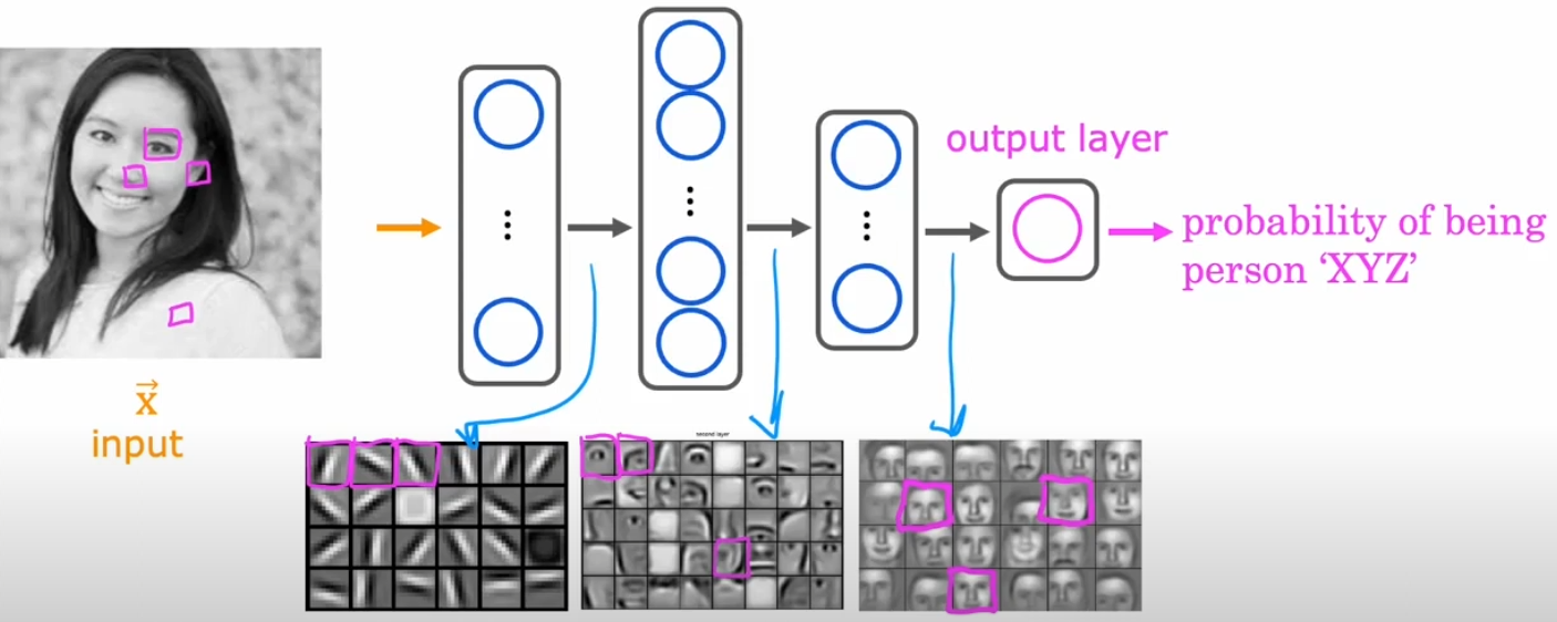
- Output Layer: Determines whether the face matches a known identity by producing a probability score.
Mathematical Representation of a Neural Network
To efficiently compute activations in a neural network, we use matrix notation. The general formula for forward propagation is:
$$ Z^{[l]} = W^{[l]} A^{[l-1]} + b^{[l]} $$
where:
- $ A^{[l-1]} $ is the activation from the previous layer,
- $ W^{[l]} $ is the weight matrix of the current layer,
- $ b^{[l]} $ is the bias vector,
- $ Z^{[l]} $ is the linear combination of inputs before applying the activation function.
The activation function is applied as:
$$ A^{[l]} = g(Z^{[l]}) $$
where $ g $ is typically a sigmoid, ReLU, or softmax function.
Example Calculation
Suppose we have a single-layer neural network with three inputs and one neuron. We define the inputs as:
$$ x_1 = 0.5, \quad x_2 = 0.8, \quad x_3 = 0.2 $$
The corresponding weight matrix and bias term are given by:
$$ W = \left[ \begin{array}{ccc} 0.9 & -0.5 & 0.3 \end{array} \right], \quad b = 0.1 $$
The weighted sum (Z) is calculated as:
$$ Z = W \cdot X + b = (0.5 \times 0.9) + (0.8 \times -0.5) + (0.2 \times 0.3) + 0.1 $$
$$ Z = 0.45 - 0.4 + 0.06 + 0.1 = 0.21 $$
Applying the sigmoid activation function:
$$ \sigma(Z) = \frac{1}{1 + e^{-Z}} = \frac{1}{1 + e^{-0.21}} \approx 0.552 $$
Since the output is above 0.5, we classify this case as positive.
Two Hidden Layer Neural Network Calculation
Now, let’s consider a neural network with two hidden layers.
Network Structure
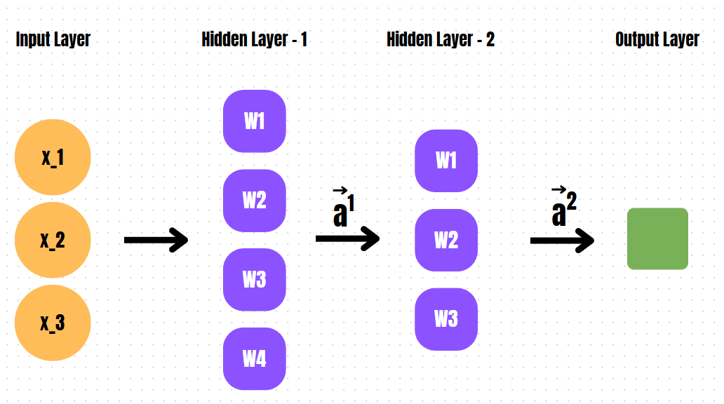
- Input Layer: 3 input values $X = [x_1, x_2, x_3]$
- First Hidden Layer: 4 neurons
- Second Hidden Layer: 3 neurons
- Output Layer: 1 neuron
First Hidden Layer Calculation
Given input vector:
$$ X = \left[ \begin{array}{c} 0.5 \ 0.8 \ 0.2 \end{array} \right] $$
Weight matrix for the first hidden layer:
$$ W^{(1)} = \left[ \begin{array}{ccc} 0.2 & -0.3 & 0.5 \ -0.7 & 0.1 & 0.4 \ 0.3 & 0.8 & -0.6 \ 0.5 & -0.2 & 0.7 \end{array} \right] $$
Bias vector:
$$ b^{(1)} = \left[ \begin{array}{c} 0.1 \ -0.2 \ 0.3 \ 0.4 \end{array} \right] $$
Computing the weighted sum:
$$ Z^{(1)} = W^{(1)}X + b^{(1)} $$
Applying the sigmoid activation function:
$$ A^{(1)} = \sigma(Z^{(1)}) $$
Second Hidden Layer Calculation
Weight matrix:
$$ W^{(2)} = \left[ \begin{array}{cccc} 0.6 & -0.1 & 0.3 & 0.7 \ 0.2 & 0.9 & -0.5 & 0.4 \ -0.3 & 0.5 & 0.7 & -0.6 \end{array} \right] $$
Bias vector:
$$ b^{(2)} = \left[ \begin{array}{c} -0.1 \ 0.3 \ 0.2 \end{array} \right] $$
Computing the weighted sum:
$$ Z^{(2)} = W^{(2)} A^{(1)} + b^{(2)} $$
Applying the sigmoid activation function:
$$ A^{(2)} = \sigma(Z^{(2)}) $$
Output Layer Calculation
Weight matrix:
$$ W^{(3)} = \left[ \begin{array}{ccc} 0.5 & -0.7 & 0.6 \end{array} \right] $$
Bias:
$$ b^{(3)} = -0.2 $$
Computing the final weighted sum:
$$ Z^{(3)} = W^{(3)} A^{(2)} + b^{(3)} $$
Applying the sigmoid activation function:
$$ A^{(3)} = \sigma(Z^{(3)}) $$
If $ A^{(3)} > 0.5 $, the output is classified as positive.
Conclusion
- The first hidden layer extracts basic features.
- The second hidden layer learns more abstract representations.
- The output layer makes the final classification decision.
This demonstrates how a multi-layer neural network processes information in a hierarchical manner.
Handwritten Digit Recognition Using Two Layers
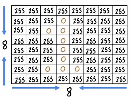
A classic application of neural networks is handwritten digit recognition. Let’s consider recognizing the digit ‘1’ from an 8x8 pixel grid using a simple neural network with two layers.
First Layer: Feature Extraction
- The 8x8 image is flattened into a 64-dimensional input vector.
- This vector is processed by neurons in the first hidden layer.
- The neurons identify edges, curves, and simple shapes using learned weights.
- Mathematically, the output of the first layer can be represented as:
$$ Z^{(1)} = W^{(1)}X + b^{(1)} $$ $$ A^{(1)} = \sigma(Z^{(1)}) $$
Second Layer: Pattern Recognition
- The first layer’s output is passed to a second hidden layer.
- This layer detects digit-specific features, such as the vertical stroke characteristic of ‘1’.
- The transformation at this stage follows:
$$ Z^{(2)} = W^{(2)}A^{(1)} + b^{(2)} $$ $$ A^{(2)} = \sigma(Z^{(2)}) $$
Output Layer: Classification
- The final layer has 10 neurons, each representing a digit from 0 to 9.
- The neuron with the highest activation determines the predicted digit:
$$ Z^{(3)} = W^{(3)}A^{(2)} + b^{(3)} $$ $$ \text{Prediction} = \arg\max(A^{(3)}) $$
This structured approach demonstrates how neural networks model real-world problems, from binary classification to deep learning applications like face and handwriting recognition.
Implementation of Forward Propagation
- Coffee Roasting Example (Classification Task)
- Neural Network Architecture
- TensorFlow Implementation
- Forward Propagation Step-by-Step (NumPy Implementation)
- Artificial General Intelligence (AGI)
Coffee Roasting Example (Classification Task)
Imagine we want to classify coffee as either “Good” or “Bad” based on two factors:
- Temperature (°C)
- Roasting Time (minutes)
For simplicity, we define:
- Good coffee: If the temperature is between 190°C and 210°C and the roasting time is between 10 and 15 minutes.
- Bad coffee: Any other condition.
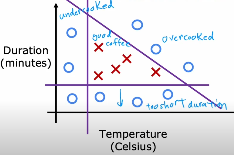
We collect the following data:
| Temperature (°C) | Roasting Time (min) | Quality (1 = Good, 0 = Bad) |
|---|---|---|
| 200 | 12 | 1 |
| 180 | 10 | 0 |
| 210 | 15 | 1 |
| 220 | 20 | 0 |
| 195 | 13 | 1 |
We will implement a simple neural network using TensorFlow to classify new coffee samples.
Neural Network Architecture
We construct a neural network using the following structure:
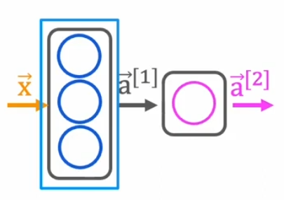
- Input Layer: Two neurons (temperature, time)
- Hidden Layer: Three neurons, activated with the sigmoid function
- Output Layer: One neuron, activated with the sigmoid function (binary classification)
TensorFlow Implementation
Step 1: Importing Libraries
import tensorflow as tf
import numpy as np
tensorflowis the core deep learning library that allows us to define and train neural networks.numpyis used for handling arrays and numerical operations efficiently.
Step 2: Defining Inputs and Outputs
X = np.array([[200, 12], [180, 10], [210, 15], [220, 20], [195, 13]], dtype=np.float32)
y = np.array([[1], [0], [1], [0], [1]], dtype=np.float32)
Xrepresents the input features (temperature and roasting time) as a NumPy array.yrepresents the expected output (1 for good coffee, 0 for bad coffee).dtype=np.float32ensures numerical stability and compatibility with TensorFlow.
Step 3: Building the Model
model = tf.keras.Sequential([
    tf.keras.layers.Dense(3, activation='sigmoid', input_shape=(2,)),
    tf.keras.layers.Dense(1, activation='sigmoid')
])
Sequential()creates a linear stack of layers.Dense(3, activation='sigmoid', input_shape=(2,))defines the hidden layer:- 3 neurons
- Sigmoid activation function
- Input shape of (2,) since we have two input features.
Dense(1, activation='sigmoid')defines the output layer with 1 neuron and sigmoid activation.
Step 4: Training the Model
model.compile(optimizer='adam', loss='binary_crossentropy', metrics=['accuracy'])
model.fit(X, y, epochs=500, verbose=0)
compile()configures the model for training:adamoptimizer adapts the learning rate automatically.binary_crossentropyis used for binary classification problems.accuracymetric tracks how well the model classifies coffee samples.
fit(X, y, epochs=500, verbose=0)trains the model for 500 epochs (iterations over data).
Step 5: Making Predictions
new_coffee = np.array([[205, 14]], dtype=np.float32)
prediction = model.predict(new_coffee)
print("Prediction (Probability of Good Coffee):", prediction)
new_coffeecontains a new sample (205°C, 14 min) to classify.model.predict(new_coffee)computes the probability of the coffee being good.- The output is a probability (closer to 1 means good, closer to 0 means bad).
Forward Propagation Step-by-Step (NumPy Implementation)
We now implement forward propagation manually using NumPy to understand how TensorFlow executes it under the hood.
Initializing Weights and Biases
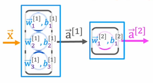
np.random.seed(42)  # For reproducibility
W1 = np.random.randn(2, 4)  # Weights for hidden layer (2 inputs -> 4 neurons)
b1 = np.random.randn(4)     # Bias for hidden layer
W2 = np.random.randn(4, 1)  # Weights for output layer (4 neurons -> 1 output)
b2 = np.random.randn(1)     # Bias for output layer
np.random.randn()initializes weights and biases randomly from a normal distribution.W1andb1define the hidden layer parameters.W2andb2define the output layer parameters.
Forward Propagation Calculation
def sigmoid(z):
    return 1 / (1 + np.exp(-z))
- This function applies the sigmoid activation function, which outputs values between 0 and 1.
def forward_propagation(X):
    Z1 = np.dot(X, W1) + b1  # Linear transformation (Hidden Layer)
    A1 = sigmoid(Z1)  # Activation function (Hidden Layer)
    Z2 = np.dot(A1, W2) + b2  # Linear transformation (Output Layer)
    A2 = sigmoid(Z2)  # Activation function (Output Layer)
    return A2
np.dot(X, W1) + b1computes the weighted sum of inputs for the hidden layer.sigmoid(Z1)applies the activation function to introduce non-linearity.np.dot(A1, W2) + b2computes the weighted sum of outputs from the hidden layer.sigmoid(Z2)produces the final prediction.
# Testing with an example input
output = forward_propagation(np.array([[185, 10]]))
print(output)
This manually replicates TensorFlow’s forward propagation but using pure NumPy.
Artificial General Intelligence (AGI)
AGI refers to AI that can perform any intellectual task a human can. Unlike current AI systems, AGI would adapt, learn, and generalize across different tasks without needing task-specific training.
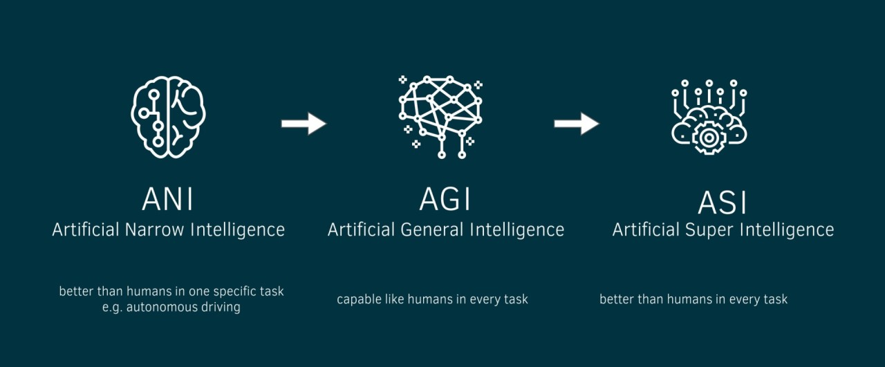
Everyday Example: AGI vs. Narrow AI
- Narrow AI (Current AI): A chess-playing AI can defeat world champions but cannot drive a car.
- AGI: If a chess-playing AI was truly intelligent, it would learn how to drive just like a human without explicit programming.
Key Challenges in AGI
- Transfer Learning: Current AI requires large amounts of data. Humans learn with few examples.
- Common Sense Reasoning: AI struggles with simple logic like “If I drop a glass, it will break.”
- Self-Learning: AGI must improve without needing human intervention.
Is AGI Possible?
- Some scientists believe AGI is decades away, while others argue it may never happen.
- Brain-inspired architectures (like Neural Networks) might be a stepping stone toward AGI.
Neural Network Training and Activation Functions
Understanding Loss Functions
Binary Crossentropy (BCE)
Binary crossentropy is commonly used for binary classification problems. It measures the difference between the predicted probability $ \hat{y} $ and the true label $ y $ as follows:
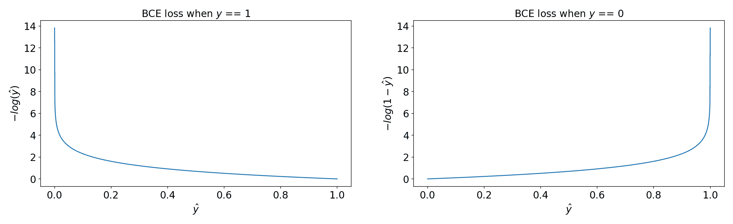
$$ L = - \frac{1}{N} \sum\limits_{i=1}^{N} \left[ y_i \log(\hat{y}_i) + (1 - y_i) \log(1 - \hat{y}_i) \right] $$
TensorFlow Implementation
import tensorflow as tf
loss_fn = tf.keras.losses.BinaryCrossentropy()
y_true = [1, 0, 1, 1]
y_pred = [0.9, 0.1, 0.8, 0.6]
loss = loss_fn(y_true, y_pred)
print("Binary Crossentropy Loss:", loss.numpy())
Mean Squared Error (MSE)
For regression problems, MSE calculates the average squared differences between actual and predicted values:
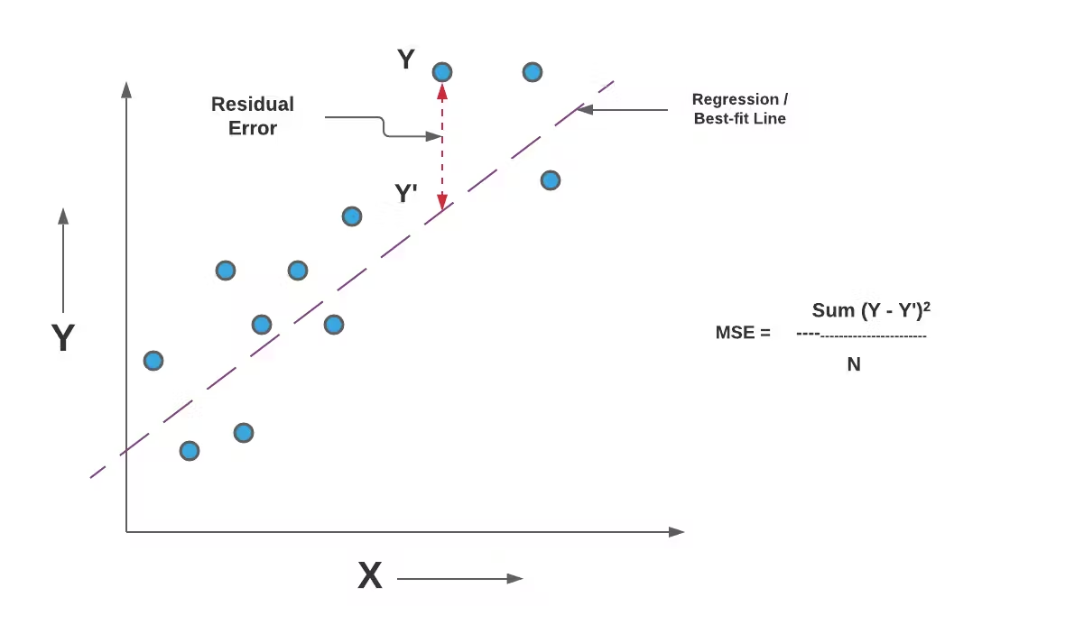
$$ L = \frac{1}{N} \sum\limits_{i=1}^{N} (y_i - \hat{y}_i)^2 $$
TensorFlow Implementation
mse_fn = tf.keras.losses.MeanSquaredError()
y_true = [3.0, -0.5, 2.0, 7.0]
y_pred = [2.5, 0.0, 2.1, 7.8]
mse_loss = mse_fn(y_true, y_pred)
print("Mean Squared Error Loss:", mse_loss.numpy())
Categorical Crossentropy (CCE)
Categorical crossentropy is used for multi-class classification problems where labels are one-hot encoded. The loss function is given by:
$$L = - \sum\limits_{i=1}^{N} \sum\limits_{j=1}^{C} y_{ij} \log(\hat{y}_{ij})$$
where $ C $ is the number of classes.
TensorFlow Implementation
cce_fn = tf.keras.losses.CategoricalCrossentropy()
y_true = [[0, 0, 1], [0, 1, 0]]  # One-hot encoded labels
y_pred = [[0.1, 0.2, 0.7], [0.2, 0.6, 0.2]]  # Model predictions
cce_loss = cce_fn(y_true, y_pred)
print("Categorical Crossentropy Loss:", cce_loss.numpy())
Sparse Categorical Crossentropy (SCCE)
Sparse categorical crossentropy is similar to categorical crossentropy but used when labels are not one-hot encoded (i.e., they are integers instead of vectors).
TensorFlow Implementation
scce_fn = tf.keras.losses.SparseCategoricalCrossentropy()
y_true = [2, 1]  # Integer labels
y_pred = [[0.1, 0.2, 0.7], [0.2, 0.6, 0.2]]  # Model predictions
scce_loss = scce_fn(y_true, y_pred)
print("Sparse Categorical Crossentropy Loss:", scce_loss.numpy())
Choosing the Right Loss Function
| Problem Type | Suitable Loss Function | Example Application |
|---|---|---|
| Binary Classification | BinaryCrossentropy | Spam detection |
| Multi-class Classification (one-hot) | CategoricalCrossentropy | Image classification |
| Multi-class Classification (integer labels) | SparseCategoricalCrossentropy | Sentiment analysis |
| Regression | MeanSquaredError | House price prediction |
Each loss function serves a different purpose and is chosen based on the nature of the problem. For classification tasks, crossentropy-based losses are preferred, while for regression, MSE is commonly used. Understanding the structure of your dataset and the expected output format is crucial when selecting the right loss function.
Training Details Main Concepts
Epochs
An epoch represents one complete pass of the entire training dataset through the neural network. During each epoch, the model updates its weights based on the error calculated from the loss function.
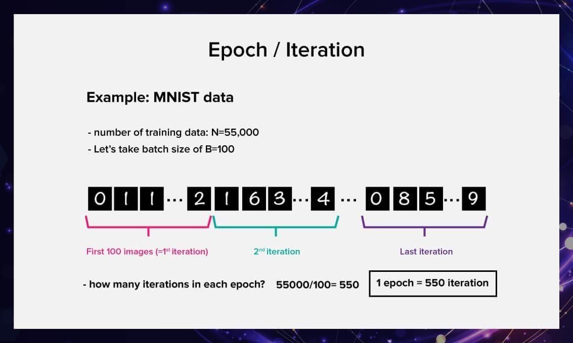
- If we train for one epoch, the model sees each training sample exactly once.
- If we train for multiple epochs, the model repeatedly sees the same data and continuously updates its weights to improve performance.
Choosing the Number of Epochs
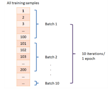
- Too Few Epochs → The model may underfit, meaning it has not learned enough patterns from the data.
- Too Many Epochs → The model may overfit, meaning it memorizes the training data but generalizes poorly to new data.
- The optimal number of epochs is typically determined using early stopping, which monitors validation loss and stops training when the loss starts increasing (a sign of overfitting).
TensorFlow Implementation
model.fit(X_train, y_train, epochs=50, batch_size=32, validation_data=(X_val, y_val))
Batch Size
Instead of feeding the entire dataset into the model at once, training is performed in smaller subsets called batches.
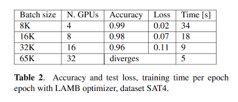
Key Concepts:
- Batch Size: The number of training samples processed before updating the model’s weights.
- Iteration: One update of the model’s weights after processing a batch.
- Steps Per Epoch: If we have
Ntraining samples and batch sizeB, then the number of steps per epoch is N/B.
Choosing Batch Size
- Small Batch Sizes (e.g., 16, 32):
- Require less memory.
- Provide noisy but effective updates (better generalization).
- Large Batch Sizes (e.g., 256, 512, 1024):
- Require more memory.
- Lead to smoother but potentially less generalized updates.
TensorFlow Implementation
model.fit(X_train, y_train, epochs=20, batch_size=64)
Validation Data
A validation set is a separate portion of the dataset that is not used for training. It helps monitor the model’s performance and detect overfitting.
Differences Between Training, Validation, and Test Data:
| Data Type | Purpose |
|---|---|
| Training Set | Used for updating model weights during training. |
| Validation Set | Used to tune hyperparameters and detect overfitting. |
| Test Set | Used to evaluate final model performance on unseen data. |
How to Split Data:
A common split is 80% training, 10% validation, 10% test, but this can vary based on dataset size.
TensorFlow Implementation
from sklearn.model_selection import train_test_split

X_train, X_val, y_train, y_val = train_test_split(X, y, test_size=0.2, random_state=42)

model.fit(X_train, y_train, epochs=30, batch_size=32, validation_data=(X_val, y_val))
Activation Functions
1. Why Do We Need Activation Functions?
Without an activation function, a neural network with multiple layers behaves like a single-layer linear model because:
$$ f(x) = Wx + b $$
is just a linear transformation. Activation functions introduce non-linearity, allowing the network to learn complex patterns.
If we do not apply non-linearity, no matter how many layers we stack, the final output remains a linear function of the input. Activation functions solve this by enabling the model to approximate complex, non-linear relationships.
2. Common Activation Functions
Sigmoid (Logistic Function)
$$ \sigma(x) = \frac{1}{1 + e^{-x}} $$
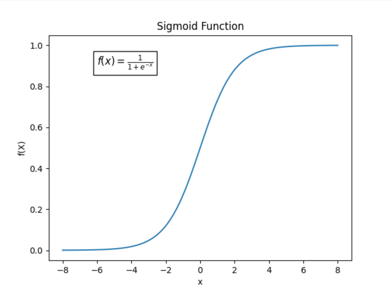
- Range: (0, 1)
- Used in: Binary classification problems
- Pros: Outputs can be interpreted as probabilities.
- Cons: Vanishing gradients for very large or very small values of ( x ), making training slow.
ReLU (Rectified Linear Unit)
$$ f(x) = \max(0, x) $$
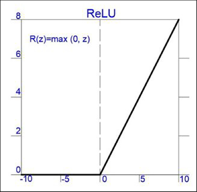
- Range: [0, ∞)
- Used in: Hidden layers of deep neural networks.
- Pros: Helps with gradient flow and avoids vanishing gradients.
- Cons: Can suffer from dying ReLU problem (where neurons output 0 and stop learning if input is negative).
Leaky ReLU
$$ f(x) = \max(0.01x, x) $$
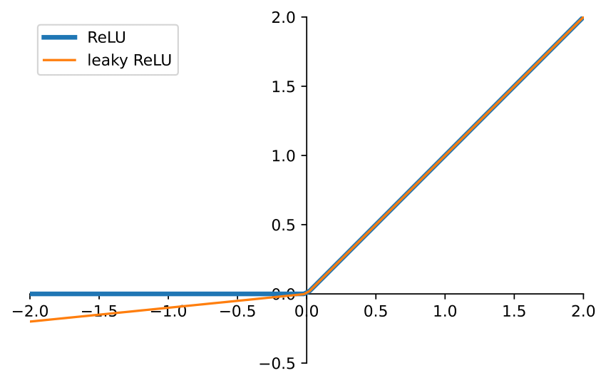
- Range: (-∞, ∞)
- Used in: Hidden layers as an alternative to ReLU.
- Pros: Prevents the dying ReLU problem.
- Cons: Small negative slope may still lead to slow learning.
Softmax
$$ \sigma(xi) = \frac{e^{x_i}}{\sum{j} e^{x_j}} $$
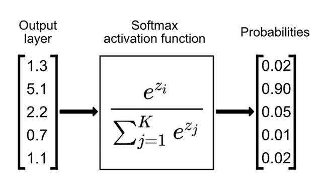
- Used in: Multi-class classification (output layer).
- Pros: Outputs a probability distribution (each class gets a probability between 0 and 1, summing to 1).
- Cons: Can lead to numerical instability when exponentiating large numbers.
Linear Activation
$$ f(x) = x $$
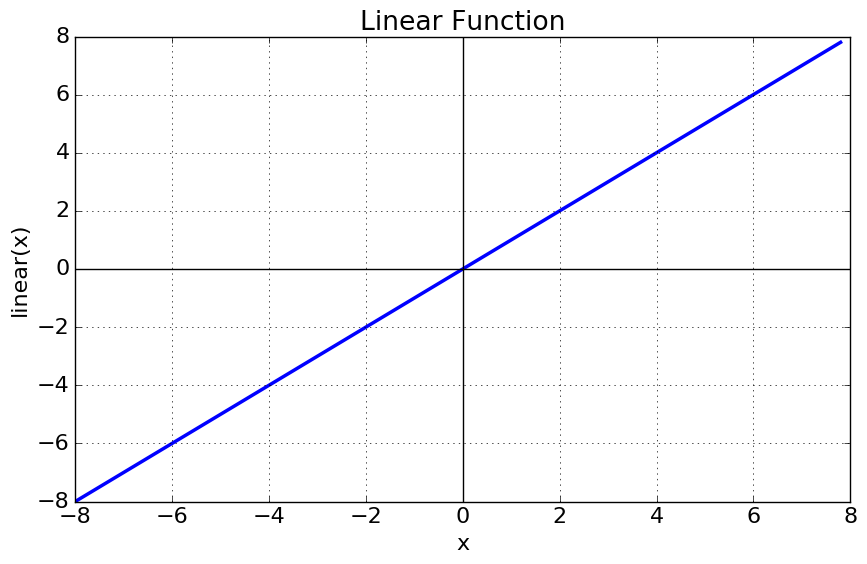
- Used in: Regression problems (output layer).
- Pros: No constraints on output values.
- Cons: Not useful for classification since it doesn’t map values to a specific range.
3. Choosing the Right Activation Function
| Layer | Recommended Activation Function | Explanation |
|---|---|---|
| Hidden Layers | ReLU (or Leaky ReLU if ReLU is dying) | Helps with deep networks by maintaining gradient flow |
| Output Layer (Binary Classification) | Sigmoid | Outputs probabilities for two-class classification |
| Output Layer (Multi-Class Classification) | Softmax | Converts logits into probability distributions |
| Output Layer (Regression) | Linear | Directly outputs numerical values |
Softmax vs. Sigmoid: Key Differences
- Sigmoid is mainly used for binary classification, mapping values to (0,1), which can be interpreted as class probabilities.
- Softmax is used for multi-class classification, producing a probability distribution over multiple classes.
If you use sigmoid for multi-class problems, each output node will act independently, making it difficult to ensure they sum to 1. Softmax ensures that outputs sum to 1, providing a clearer probabilistic interpretation.
Improved Implementation of Softmax
Why Use Linear Instead of Softmax in the Output Layer?
When implementing a neural network for classification, we often pass logits (raw outputs) directly into the loss function instead of applying softmax explicitly.
Mathematically, if we apply softmax explicitly:
$$ L = - \sum y_i \log(\sigma(z_i)) $$
where ( \sigma(z) ) is the softmax function.
However, if we pass raw logits (without softmax) into the cross-entropy loss function, TensorFlow applies the log-softmax trick internally:
$$ L = - \sum y_i z_i + \log \sum e^{z_i} $$
This avoids computing large exponentials, improving numerical stability and reducing computation cost.
TensorFlow Implementation
Instead of:
model = tf.keras.Sequential([
    tf.keras.layers.Dense(128, activation='relu'),
    tf.keras.layers.Dense(64, activation='relu'),
    tf.keras.layers.Dense(10, activation='softmax')  # Explicit softmax
])
model.compile(loss=tf.keras.losses.SparseCategoricalCrossentropy(), optimizer='adam')
Use:
model = tf.keras.Sequential([
    tf.keras.layers.Dense(128, activation='relu'),
    tf.keras.layers.Dense(64, activation='relu'),
    tf.keras.layers.Dense(10)  # No activation here!
])
model.compile(loss=tf.keras.losses.SparseCategoricalCrossentropy(from_logits=True), optimizer='adam')
This allows TensorFlow to handle softmax internally, avoiding unnecessary computation and improving numerical precision.
Optimizers and Layer Types
- Optimizers in Deep Learning
- Choosing the Right Optimizer
- Gradient Descent (GD)
- Stochastic Gradient Descent (SGD)
- Stochastic Gradient Descent with Momentum (SGD-Momentum)
- Mini-Batch Gradient Descent
- Adagrad (Adaptive Gradient Descent)
- RMSprop (Root Mean Square Propagation)
- AdaDelta
- Adam (Adaptive Moment Estimation)
- Hands-on Optimizers
- Table Analysis
- Conclusion
- Additional Layer Types in Neural Networks
Optimizers in Deep Learning
Optimizers play a crucial role in training deep learning models by adjusting the model parameters to minimize the loss function. Different optimization algorithms have been developed to improve convergence speed, accuracy, and stability. In this article, we explore various optimizers used in deep learning, their mathematical formulations, and practical implementations.
Choosing the Right Optimizer
Choosing the right optimizer depends on several factors, including:
- The nature of the dataset
- The complexity of the model
- The presence of noisy gradients
- The required computational efficiency
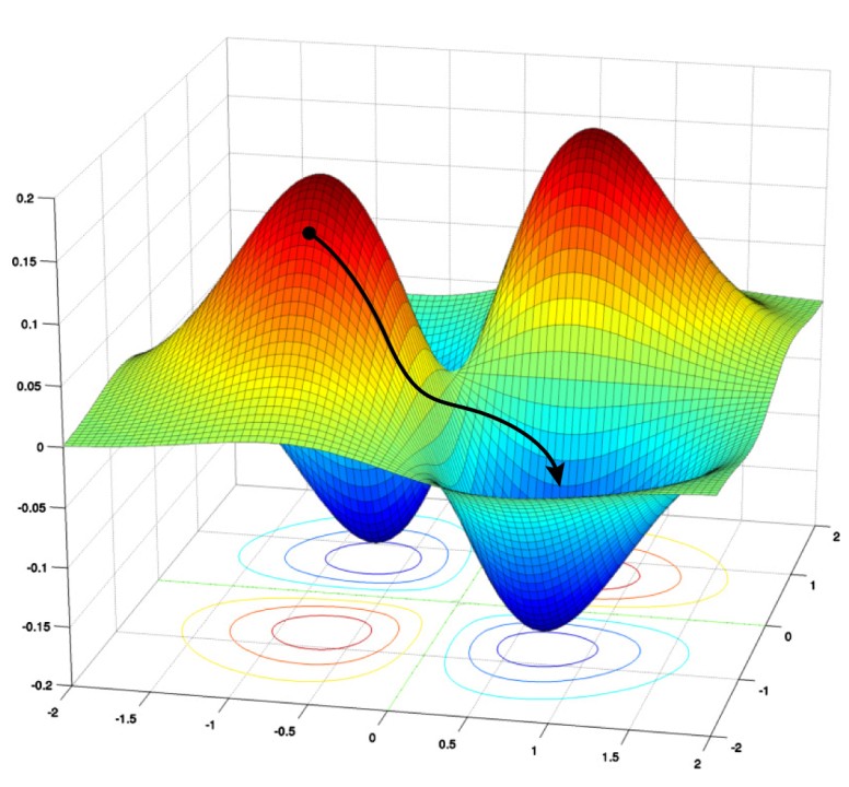
Below, we examine different types of optimizers along with their mathematical formulations.
Gradient Descent (GD)
Mathematical Formulation
Gradient Descent updates model parameters $ \theta $ iteratively using the gradient of the loss function $ J(\theta) $:
$$ \theta = \theta - \alpha \nabla J(\theta) $$
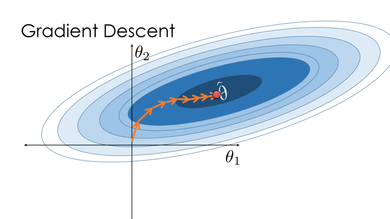
where:
- $ \alpha $ is the learning rate
- $ \nabla J(\theta) $ is the gradient of the loss function
Characteristics
- Computes gradient over the entire dataset
- Slow for large datasets
- Prone to getting stuck in local minima
Stochastic Gradient Descent (SGD)
Gradient descent struggles with massive datasets, making stochastic gradient descent (SGD) a better alternative. Unlike standard gradient descent, SGD updates model parameters using small, randomly selected data batches, improving computational efficiency.
SGD initializes parameters $𝑤$ and learning rate $\alpha$, then shuffles data at each iteration, updating based on mini-batches. This introduces noise, requiring more iterations to converge, but still reduces overall computation time compared to full-batch gradient descent.
For large datasets where speed matters, SGD is preferred over batch gradient descent.
Mathematical Formulation
Instead of computing the gradient over the entire dataset, SGD updates $ \theta $ using a single data point:
$$ \theta = \theta - \alpha \nabla J(\theta; x_i, y_i) $$
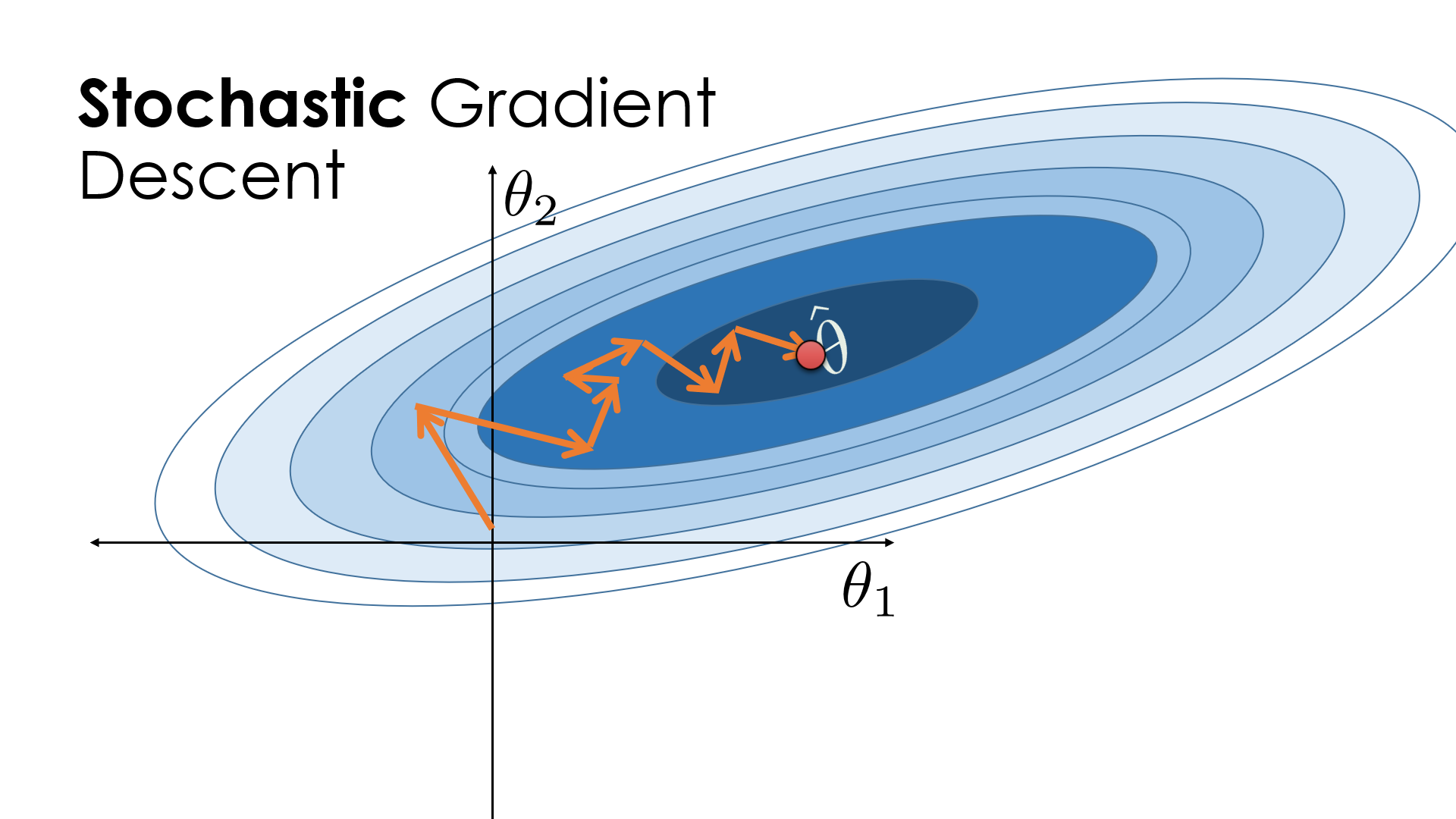
where $ x_i, y_i $ is a single training example.
Characteristics
- Faster than full-batch gradient descent
- High variance in updates
- Introduces noise, which can help escape local minima
Stochastic Gradient Descent with Momentum (SGD-Momentum)
SGD follows a noisy optimization path, requiring more iterations and longer computation time. To speed up convergence, SGD with momentum is used.
Momentum helps stabilize updates by adding a fraction of the previous update to the current one, reducing oscillations and accelerating convergence. However, a high momentum term requires lowering the learning rate to avoid overshooting the optimal minimum.
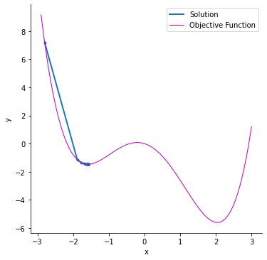
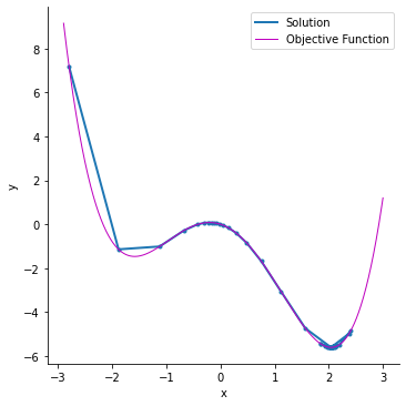
While momentum improves speed, too much momentum can cause instability and poor accuracy. Proper tuning is essential for effective optimization.
Mathematical Formulation
Momentum helps accelerate SGD by maintaining a velocity term:
$$ v_t = \beta v_{t-1} + (1 - \beta) \nabla J(\theta) $$
$$ \theta = \theta - \alpha v_t $$
where:
- $ v_t $ is the momentum term
- $ \beta $ is a momentum coefficient (typically 0.9)
Characteristics
- Reduces oscillations
- Faster convergence
Mini-Batch Gradient Descent
Mini-batch gradient descent optimizes training by using a subset of data instead of the entire dataset, reducing the number of iterations needed. This makes it faster than both stochastic and batch gradient descent while being more efficient and memory-friendly.
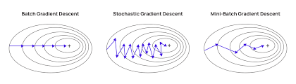
Key Advantages
- Balances speed and accuracy by reducing noise compared to SGD but keeping updates more dynamic than batch gradient descent.
- Doesn’t require loading all data into memory, improving implementation efficiency.
Limitations
- Requires tuning the mini-batch size (typically 32) for optimal accuracy.
- May lead to poor final accuracy in some cases, requiring alternative approaches.
Mathematical Formulation
$$ \theta = \theta - \alpha \frac{1}{m} \sum\limits_{i=1}^{m} \nabla J(\theta; x_i, y_i) $$
Instead of updating with the entire dataset or a single example, mini-batch GD uses a small batch of $ m $ samples:
Adagrad (Adaptive Gradient Descent)
Adagrad differs from other gradient descent algorithms by using a unique learning rate for each iteration, adjusting based on parameter changes. Larger parameter updates lead to smaller learning rate adjustments, making it effective for datasets with both sparse and dense features.
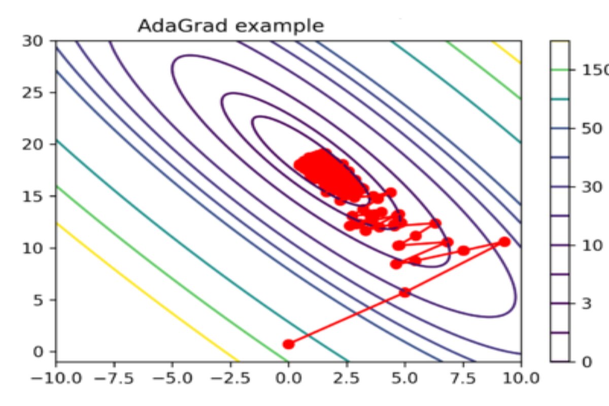
Key Advantages
- Eliminates manual learning rate tuning by adapting automatically.
- Faster convergence compared to standard gradient descent methods.
Limitations
- Aggressively reduces the learning rate over time, which can slow learning and harm accuracy.
- The accumulation of squared gradients in the denominator causes the learning rate to become too small, limiting further model improvements.
Mathematical Formulation
Adagrad adapts learning rates for each parameter:
$$ \theta = \theta - \frac{\alpha}{\sqrt{G*{t} + \epsilon}} \nabla J(\theta) $$
where $ G_t $ accumulates past squared gradients:
$$ G_t = G_{t-1} + \nabla J(\theta)^2 $$
Characteristics
- Suitable for sparse data
- Learning rate decreases over time
RMSprop (Root Mean Square Propagation)
RMSProp improves stability by adapting step sizes per weight, preventing large gradient fluctuations. It maintains a moving average of squared gradients to adjust learning rates dynamically.
Mathematical Formulation
$$ G_t = \beta G_{t-1} + (1 - \beta) \nabla J(\theta)^2 $$
$$ \theta = \theta - \frac{\alpha}{\sqrt{G_{t} + \epsilon}} \nabla J(\theta) $$
Pros
- Faster convergence with smoother updates.
- Less tuning than other gradient descent variants.
- More stable than Adagrad by preventing extreme learning rate decay.
Cons
- Requires manual learning rate tuning, and default values may not always be optimal.
AdaDelta
Mathematical Formulation
AdaDelta modifies Adagrad by using an exponentially decaying average of past squared gradients:
$$ \Delta \theta_t = - \frac{\sqrt{E[\Delta \theta^2] + \epsilon}}{\sqrt{E[g^2] + \epsilon}} g_t $$
where $ E[\cdot] $ is the moving average.
Characteristics
- Addresses diminishing learning rates in Adagrad
- No need to manually set a learning rate
Adam (Adaptive Moment Estimation)
Adam (Adaptive Moment Estimation) is a widely used deep learning optimizer that extends SGD by dynamically adjusting learning rates for each weight. It combines AdaGrad and RMSProp to balance adaptive learning rates and stable updates.
Mathematical Formulation
Adam combines momentum and RMSprop:
$$ m_t = \beta_1 m_{t-1} + (1 - \beta*1) \nabla J(\theta) $$
$$ v_t = \beta_2 v_{t-1} + (1 - \beta_2) \nabla J(\theta)^2 $$
$$ \theta = \theta - \alpha \frac{\hat{m_t}}{\sqrt{\hat{v_t}} + \epsilon} $$
where $ \hat{m_t} $ and $ \hat{v_t} $ are bias-corrected estimates.
Key Features
- Uses first (mean) and second (variance) moments of gradients.
- Faster convergence with minimal tuning.
- Low memory usage and efficient computation.
Downsides
- Prioritizes speed over generalization, making SGD better for some cases.
- May not always be ideal for every dataset.
Adam is the default choice for many deep learning tasks but should be selected based on the dataset and training requirements.
Hands-on Optimizers
Import Necessary Libraries
import keras
from keras.datasets import mnist
from keras.models import Sequential
from keras.layers import Dense, Dropout, Flatten
from keras.layers import Conv2D, MaxPooling2D
from keras import backend as K
(x_train, y_train), (x_test, y_test) = mnist.load_data()
print(x_train.shape, y_train.shape)
Load the Dataset
x_train= x_train.reshape(x_train.shape[0],28,28,1)
x_test=  x_test.reshape(x_test.shape[0],28,28,1)
input_shape=(28,28,1)
y_train=keras.utils.to_categorical(y_train)#,num_classes=)
y_test=keras.utils.to_categorical(y_test)#, num_classes)
x_train= x_train.astype('float32')
x_test= x_test.astype('float32')
x_train /= 255
x_test /=255
Build the Model
batch_size=64

num_classes=10

epochs=10

def build_model(optimizer):

    model=Sequential()

    model.add(Conv2D(32,kernel_size=(3,3),activation='relu',input_shape=input_shape))

    model.add(MaxPooling2D(pool_size=(2,2)))

    model.add(Dropout(0.25))

    model.add(Flatten())

    model.add(Dense(256, activation='relu'))

    model.add(Dropout(0.5))

    model.add(Dense(num_classes, activation='softmax'))

    model.compile(loss=keras.losses.categorical_crossentropy, optimizer= optimizer, metrics=['accuracy'])

    return model
Train the Model
optimizers = ['Adadelta', 'Adagrad', 'Adam', 'RMSprop', 'SGD']

for i in optimizers:

model = build_model(i)

hist=model.fit(x_train, y_train, batch_size=batch_size, epochs=epochs, verbose=1, validation_data=(x_test,y_test))
Table Analysis
| Optimizer | Epoch 1 (Val Acc | Val Loss) | Epoch 5 (Val Acc | Val Loss) | Epoch 10 (Val Acc | Val Loss) | Total Time |
|---|---|---|---|---|---|---|---|
| Adadelta | .4612 | 2.2474 | .7776 | 1.6943 | .8375 | 0.9026 | 8:02 min |
| Adagrad | .8411 | .7804 | .9133 | .3194 | .9286 | 0.2519 | 7:33 min |
| Adam | .9772 | .0701 | .9884 | .0344 | .9908 | .0297 | 7:20 min |
| RMSprop | .9783 | .0712 | .9846 | .0484 | .9857 | .0501 | 10:01 min |
| SGD with momentum | .9168 | .2929 | .9585 | .1421 | .9697 | .1008 | 7:04 min |
| SGD | .9124 | .3157 | .9569 | 1.451 | .9693 | .1040 | 6:42 min |
The above table shows the validation accuracy and loss at different epochs. It also contains the total time that the model took to run on 10 epochs for each optimizer. From the above table, we can make the following analysis.
- The adam optimizer shows the best accuracy in a satisfactory amount of time.
- RMSprop shows similar accuracy to that of Adam but with a comparatively much larger computation time.
- Surprisingly, the SGD algorithm took the least time to train and produced good results as well. But to reach the accuracy of the Adam optimizer, SGD will require more iterations, and hence the computation time will increase.
- SGD with momentum shows similar accuracy to SGD with unexpectedly larger computation time. This means the value of momentum taken needs to be optimized.
- Adadelta shows poor results both with accuracy and computation time.
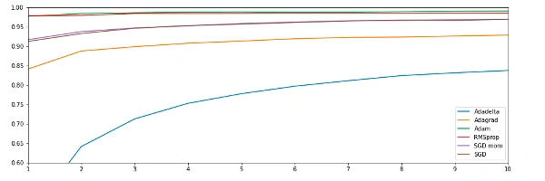
You can analyze the accuracy of each optimizer with each epoch from the above graph.
Conclusion
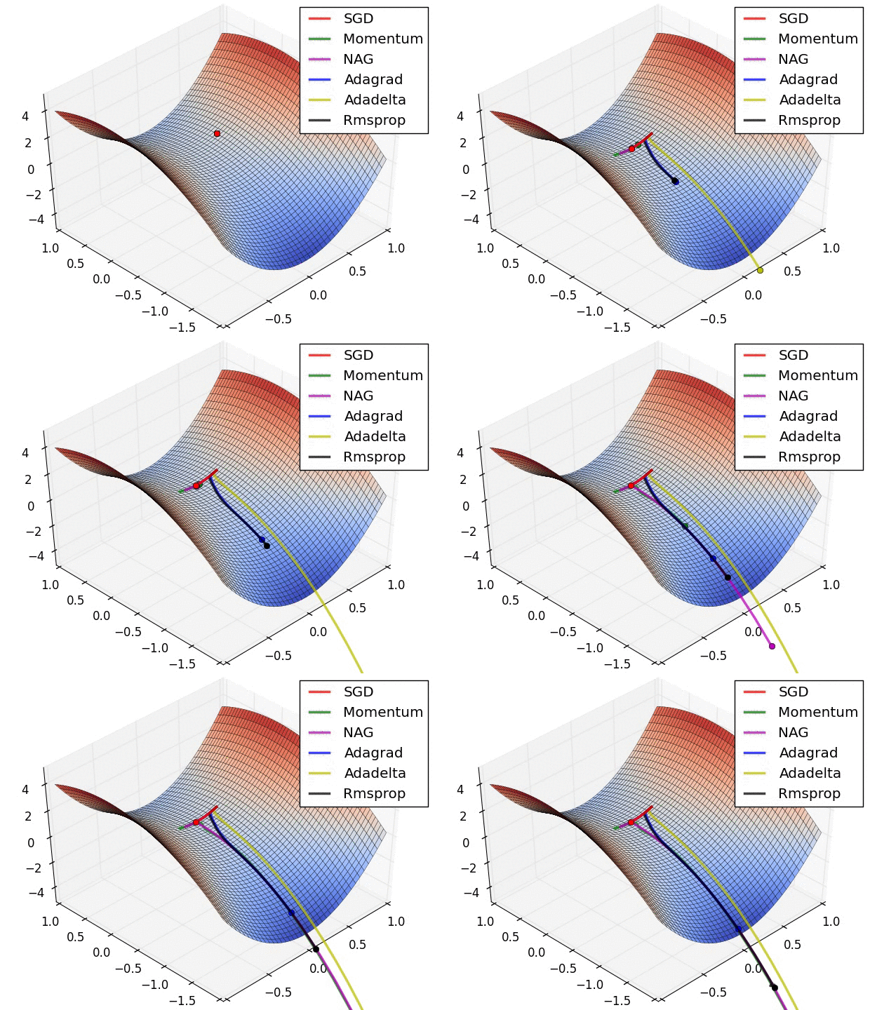
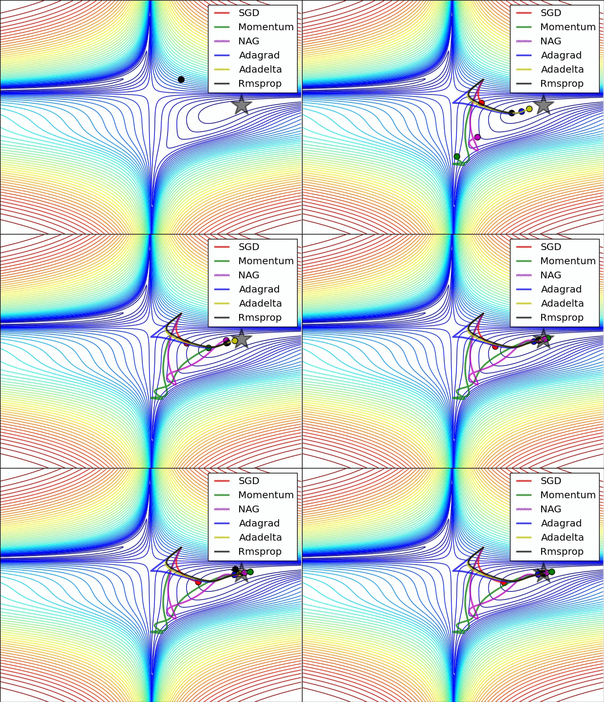
Different optimizers offer unique advantages based on the dataset and model architecture. While SGD is the simplest, Adam is often preferred for deep learning tasks due to its adaptive learning rate and momentum.
By understanding these optimizers, you can fine-tune deep learning models for optimal performance!
Additional Layer Types in Neural Networks
In deep learning, different layer types serve distinct purposes, helping neural networks learn complex representations. This section explores various layer types, their mathematical foundations, and practical implementations.
Dense Layer (Fully Connected Layer)
A Dense layer is a fundamental layer where each neuron is connected to every neuron in the previous layer.
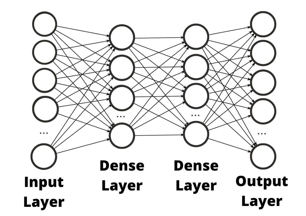
Mathematical Representation:
Given an input vector $ x $ of size $ n $, weights $ W $ of size $ m \times n $, and bias $ b $ of size $ m $, the output $ y $ is calculated as:
$$ y = f(Wx + b) $$
where $ f $ is an activation function such as ReLU, Sigmoid, or Softmax.
Implementation in TensorFlow:
import tensorflow as tf
from tensorflow.keras.models import Sequential
from tensorflow.keras.layers import Dense

model = Sequential([
    Dense(64, activation='relu', input_shape=(100,)),
    Dense(32, activation='relu'),
    Dense(10, activation='softmax')
])
model.summary()
Convolutional Layer (Conv2D)
A Convolutional layer is used in image processing, applying filters (kernels) to extract features from input images.
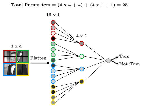
Mathematical Representation:
For an input image $ I $ and a filter $ K $, the convolution operation is defined as:
$$ S(i, j) = \sum_m \sum_n I(i+m, j+n) K(m, n) $$
Implementation in TensorFlow:
from tensorflow.keras.layers import Conv2D

model = Sequential([
    Conv2D(32, kernel_size=(3,3), activation='relu', input_shape=(28,28,1)),
    Conv2D(64, kernel_size=(3,3), activation='relu'),
])
model.summary()
Pooling Layer (MaxPooling & AveragePooling)
Pooling layers reduce dimensionality while preserving important features.
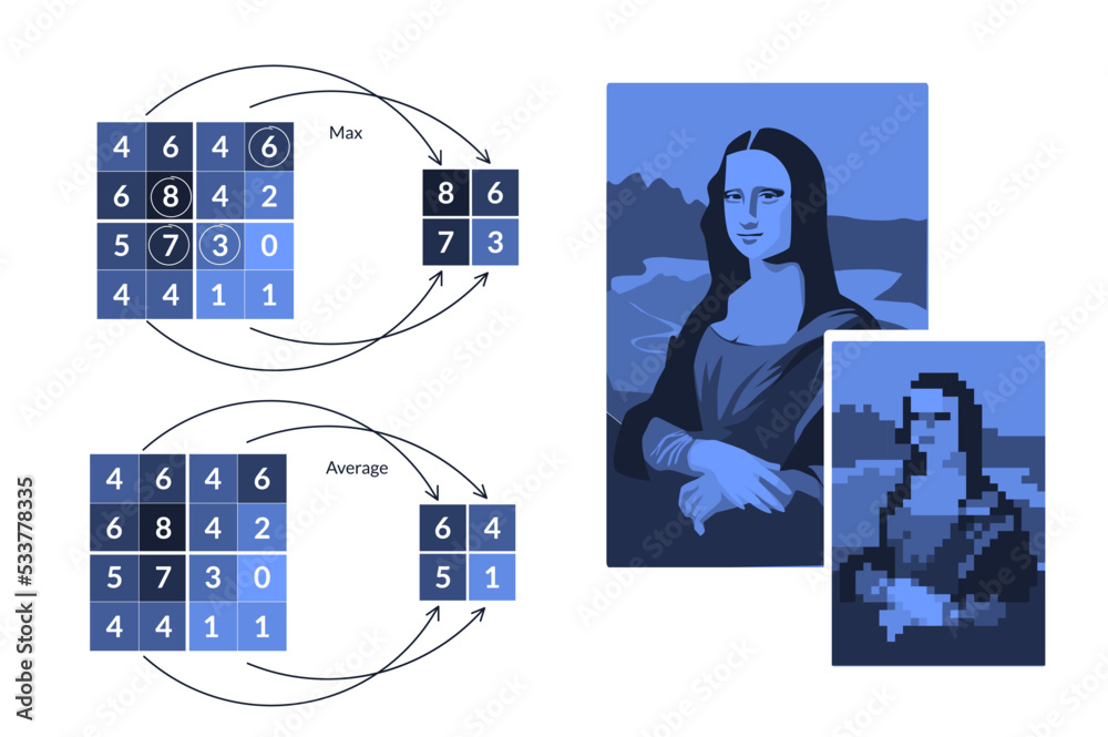
Max Pooling:
$$ S(i, j) = \max (I_{region}) $$
Average Pooling:
$$ S(i, j) = \frac{1}{N} \sum I_{region} $$
Implementation:
from tensorflow.keras.layers import MaxPooling2D, AveragePooling2D

model = Sequential([
    MaxPooling2D(pool_size=(2,2)),
    AveragePooling2D(pool_size=(2,2))
])
model.summary()
Recurrent Layer (RNN, LSTM, GRU)
Recurrent layers process sequential data by maintaining memory of past inputs.
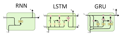
RNN Mathematical Model:
$$ h_t = f(W_h h_{t-1} + W_x x_t + b) $$
LSTM Update Equations:
$$ i_t = \sigma(W_i x_t + U_i h_{t-1} + b_i) $$
$$ f_t = \sigma(W_f x_t + U_f h_{t-1} + b_f) $$
$$ c_t = f_t c_{t-1} + i_t \tanh(W_c x_t + U_c h_{t-1} + b_c) $$
Implementation:
from tensorflow.keras.layers import SimpleRNN, LSTM, GRU

model = Sequential([
    LSTM(64, return_sequences=True, input_shape=(100, 10)),
    GRU(32)
])
model.summary()
Dropout Layer
The Dropout layer randomly sets a fraction of input units to 0 to prevent overfitting.
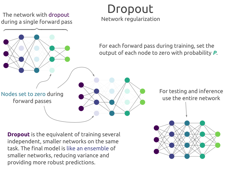
Mathematical Explanation:
During training, for each neuron, the probability of being kept is $ p $:
$$ y = \frac{1}{p} f(Wx + b) \quad \text{if neuron is kept, else } y = 0 $$
Implementation:
from tensorflow.keras.layers import Dropout

model = Sequential([
    Dense(128, activation='relu'),
    Dropout(0.5),
    Dense(64, activation='relu'),
    Dropout(0.3),
    Dense(10, activation='softmax')
])
model.summary()
Comparison Table
| Layer Type | Purpose | Typical Use Case |
|---|---|---|
| Dense | Fully connected layer | General deep learning models |
| Conv2D | Feature extraction | Image processing |
| Pooling | Downsampling | CNNs to reduce size |
| RNN | Sequential processing | Time-series, NLP |
| LSTM/GRU | Long-term memory retention | Language models |
| Dropout | Overfitting prevention | Regularization in deep networks |
Conclusion
Understanding different types of layers is crucial in designing effective deep learning models. Choosing the right layers based on the data type and problem domain significantly impacts model performance. Experimenting with combinations of these layers is key to optimizing results.
Model Evaluation, Selection, and Improvement
- Evaluating a Model
- Model Selection and Training/Validation/Test Sets
- Diagnosing Bias and Variance
- Regularization and Bias-Variance Tradeoff
- Establishing a Baseline Level of Performance
- Iterative Loop of ML Development
- Adding Data: Data Augmentation & Synthesis
- Transfer Learning: Using Data from a Different Task
- Error Metrics for Skewed Datasets
Evaluating a Model
A metric is a numerical measure used to assess the performance of a model on a given dataset. Metrics help quantify how well a model is making predictions and whether it meets the desired objectives. The choice of metric depends on the nature of the problem:
- For classification tasks, we often measure how accurately a model assigns labels.
- For regression tasks, we evaluate how close the model’s predictions are to actual values.
- In other domains like natural language processing (NLP) or computer vision, specialized metrics are used.
However, a high metric value does not always mean a model is truly effective. For example:
- In an imbalanced dataset, accuracy might be misleading. A model predicting the majority class 100% of the time can have high accuracy but perform poorly overall.
- A regression model with a low mean squared error (MSE) might still fail in real-world applications if it makes large errors in critical cases.
Key Metrics for Model Evaluation
Classification Metrics
- Accuracy: Measures the percentage of correctly predicted instances.
- Precision: The fraction of true positive predictions among all positive predictions.
- Recall: The fraction of actual positives correctly identified.
- F1-score: The harmonic mean of precision and recall, useful for imbalanced datasets.
- ROC-AUC (Receiver Operating Characteristic - Area Under Curve): Evaluates the model’s ability to distinguish between classes.
Regression Metrics
- Mean Squared Error (MSE): Measures the average squared difference between predicted and actual values.
- Mean Absolute Error (MAE): Measures the average absolute difference.
- R-squared (R²): Indicates how well the model explains variance in the data.
Other Metrics
- Log loss: Used for probabilistic classification models.
- BLEU score: Measures similarity in NLP tasks.
- Intersection over Union (IoU): Used in object detection to measure overlap between predicted and actual bounding boxes.
Choosing the Right Metric
Suppose we are building a spam classifier. If 99% of emails are non-spam, a naive model predicting “not spam” for all emails will have 99% accuracy but be completely useless. In this case, precision and recall are more meaningful metrics because they tell us how well the model detects actual spam emails without too many false positives.
Thus, choosing the right metric is just as important as achieving a high score. A well-performing model is one that aligns with the real-world objective of the task.
Model Selection and Training/Validation/Test Sets
Selecting the right model is essential for achieving high performance on unseen data. A model that performs well on training data but poorly on new data is overfitting, while a model that is too simple may underfit. To properly evaluate a model and fine-tune its performance, we split the dataset into three key subsets:
Training Set
The training set is the portion of the data used to train the machine learning model. The model learns patterns from this data by adjusting its internal parameters. However, evaluating the model only on the training set is misleading because the model might memorize the data instead of generalizing from it.
Validation Set
The validation set is a separate portion of the dataset that is used to tune hyperparameters and select the best model architecture. Hyperparameters are external configuration settings that are not learned by the model but instead set manually or through automated search methods. Examples of hyperparameters include:
- Learning rate
- Number of hidden layers in a neural network
- Regularization parameters (L1, L2)
- Batch size
By testing different hyperparameter values on the validation set, we can find the combination that leads to the best generalization performance. However, if the validation set is too small or used excessively for tuning, the model might start overfitting to it.
Test Set
The test set is used only once, after model training and hyperparameter tuning, to evaluate the final model’s performance. The test set should remain completely unseen during training and validation to provide an unbiased estimate of how the model will perform on real-world data.
Cross-Validation
Cross-validation is a technique to make better use of available data and improve model selection. Instead of relying on a single validation set, we divide the dataset into multiple subsets and perform training and validation multiple times. The most common approach is k-fold cross-validation, which works as follows:
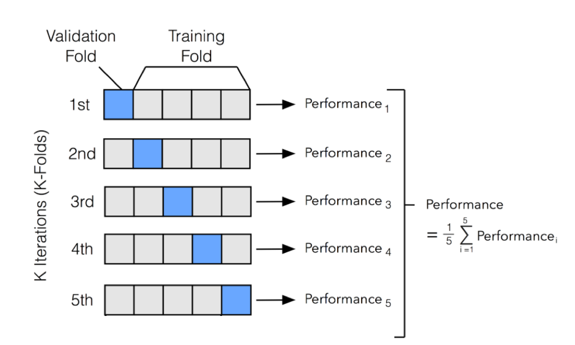
- The dataset is divided into k equal-sized folds.
- The model is trained on k-1 folds and validated on the remaining one.
- This process is repeated k times, with each fold serving as the validation set once.
- The final performance metric is the average of all validation scores.
For example, in 5-fold cross-validation, the dataset is split into 5 parts. The model is trained on 4 parts and validated on the remaining one, and this process repeats until each part has been used as a validation set once. This reduces the risk of selecting a model that performs well on just one specific validation set but poorly on unseen data.
Cross-validation is especially useful when working with small datasets since it allows more efficient use of data. However, it can be computationally expensive, especially for deep learning models, where training is time-consuming.
By using training, validation, and test sets appropriately—along with cross-validation where necessary—we can make informed decisions about model selection and ensure good generalization to new data.
Diagnosing Bias and Variance
Bias and variance are two key factors that determine a model’s ability to generalize to unseen data. To understand these concepts, let’s analyze the simple linear model:
$$ f(x) = wx + b $$
A well-performing model should generalize well, meaning it captures the essential patterns in the data without memorizing noise. Let’s break this down using the equation.
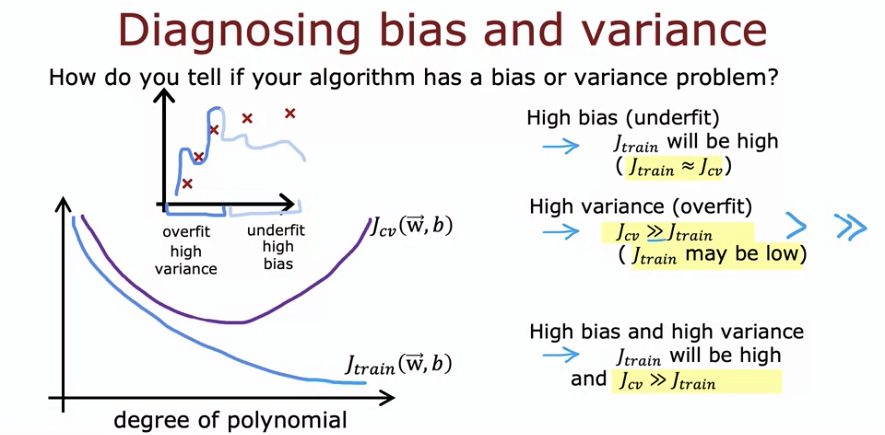
| Issue | Description | Effects | Impact of More Data |
|---|---|---|---|
| High Bias (Underfitting) | Model is too simple and cannot capture underlying patterns. | - Poor performance on both training and test sets. - Model is too simplistic. | Increasing training data does not improve performance. |
| High Variance (Overfitting) | Model is too complex and memorizes training data, including noise. | - Training error is very low, but test error is high. - Model learns noise instead of actual patterns. | Increasing training data can help generalization. |
Regularization and Bias-Variance Tradeoff
To prevent overfitting, we introduce regularization, which penalizes large weights.
The regularized loss function:
$$ J(w) = \text{Loss}(w) + \lambda \sum_{i} \phi(w_i) $$
where:
- $ \text{Loss}(w) $ is the original loss function (e.g., Mean Squared Error),
- $ \lambda $ is the regularization strength,
- $ \phi(w) $ is the penalty term (L1 or L2).
Effect of Regularization
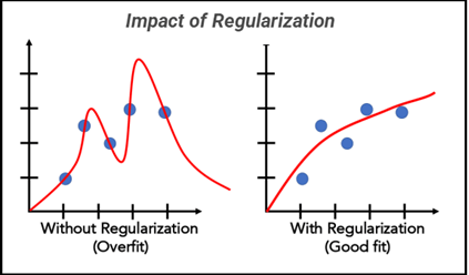
- If $ \lambda $ is too low, the model can overfit ($ w $ values become large).
- If $ \lambda $ is too high, the model becomes too simple ($ w $ values shrink too much).
- The ideal $ \lambda $ value balances bias and variance.
Establishing a Baseline Level of Performance
A baseline model helps measure improvement. Common baselines include:
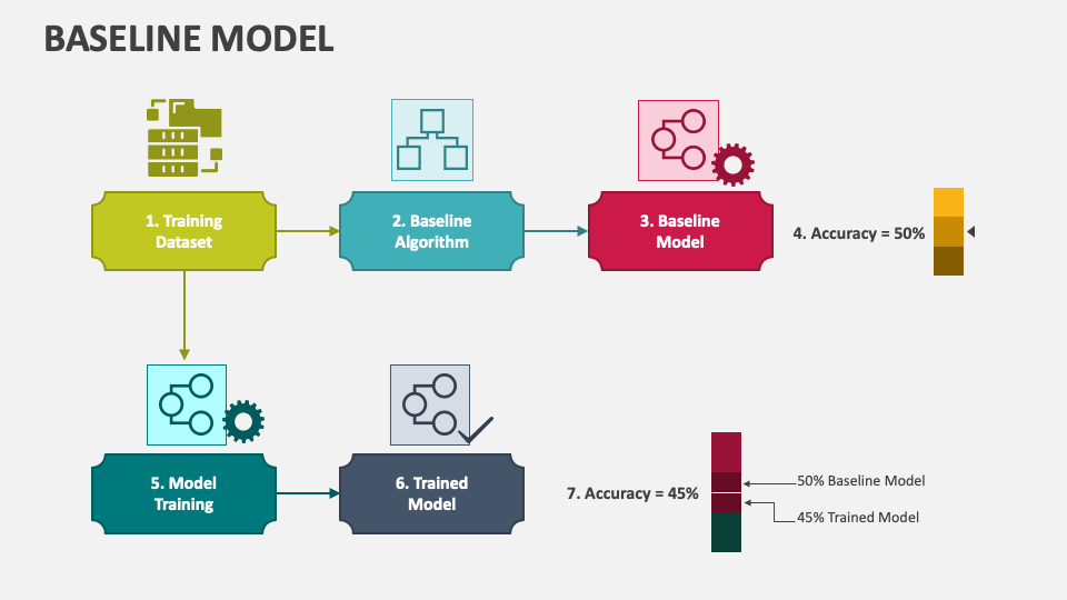
- Random classifiers (for classification tasks)
- Mean predictions (for regression tasks)
- Simple heuristic-based methods
A model must outperform the baseline to be considered useful.
Iterative Loop of ML Development
Machine learning development follows an iterative cycle:
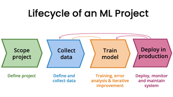
- Train a baseline model.
- Diagnose bias/variance errors.
- Adjust model complexity, regularization, or data strategy.
- Repeat until performance is satisfactory.
Adding Data: Data Augmentation & Synthesis
One of the most effective ways to improve a model’s generalization ability is by increasing the amount of training data. More data helps the model learn patterns that are not specific to the training set, reducing overfitting and improving robustness.
Data Augmentation
Data Augmentation refers to artificially increasing the size of the training dataset by applying transformations to existing data. It is particularly useful in fields like computer vision and NLP, where collecting labeled data is expensive and time-consuming.
Common Data Augmentation Techniques
-
Image Data Augmentation (Used in deep learning for computer vision tasks):
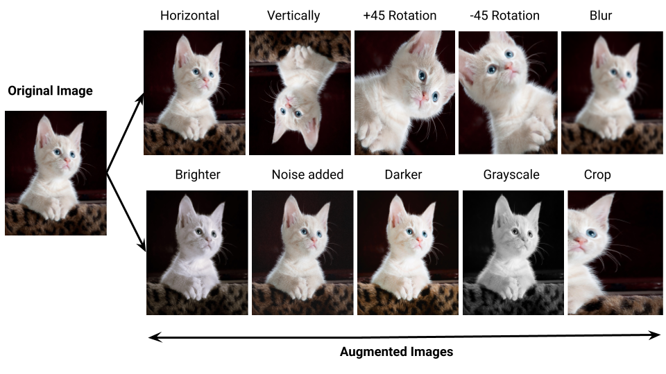
- Rotation: Rotating images by small degrees to simulate different perspectives.
- Cropping: Randomly cropping parts of the image to focus on different areas.
- Flipping: Horizontally or vertically flipping images.
- Scaling: Resizing images while maintaining aspect ratios.
- Brightness/Contrast Adjustments: Modifying brightness and contrast to simulate lighting variations.
- Noise Injection: Adding Gaussian noise to simulate different sensor conditions.
Example in TensorFlow/Keras:
from tensorflow.keras.preprocessing.image import ImageDataGenerator datagen = ImageDataGenerator( rotation_range=20, width_shift_range=0.1, height_shift_range=0.1, horizontal_flip=True, brightness_range=[0.8, 1.2] ) augmented_images = datagen.flow(x_train, y_train, batch_size=32) -
Text Data Augmentation (Used in NLP models):
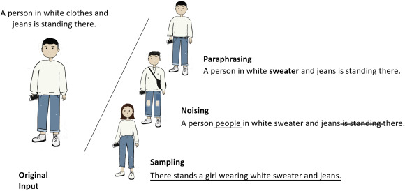
-
Synonym Replacement: Replacing words with their synonyms.
-
Random Insertion: Adding random words from the vocabulary.
-
Back Translation: Translating text to another language and back to introduce variation.
-
Sentence Shuffling: Reordering words or sentences slightly.
Example using
nlpaug:
import nlpaug.augmenter.word as naw aug = naw.SynonymAug(aug_src='wordnet') text = "Deep learning models require large amounts of data." augmented_text = aug.augment(text) print(augmented_text) -
-
Time-Series Data Augmentation (Used in financial data, speech processing):
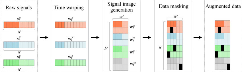
- Time Warping: Stretching or compressing time series data.
- Jittering: Adding small random noise to numerical values.
- Scaling: Multiplying data points by a random factor.
Data Synthesis
Data Synthesis involves generating entirely new data points that mimic real-world distributions. This is useful when real data is scarce or difficult to obtain.
Common Data Synthesis Techniques
-
Generative Adversarial Networks (GANs)
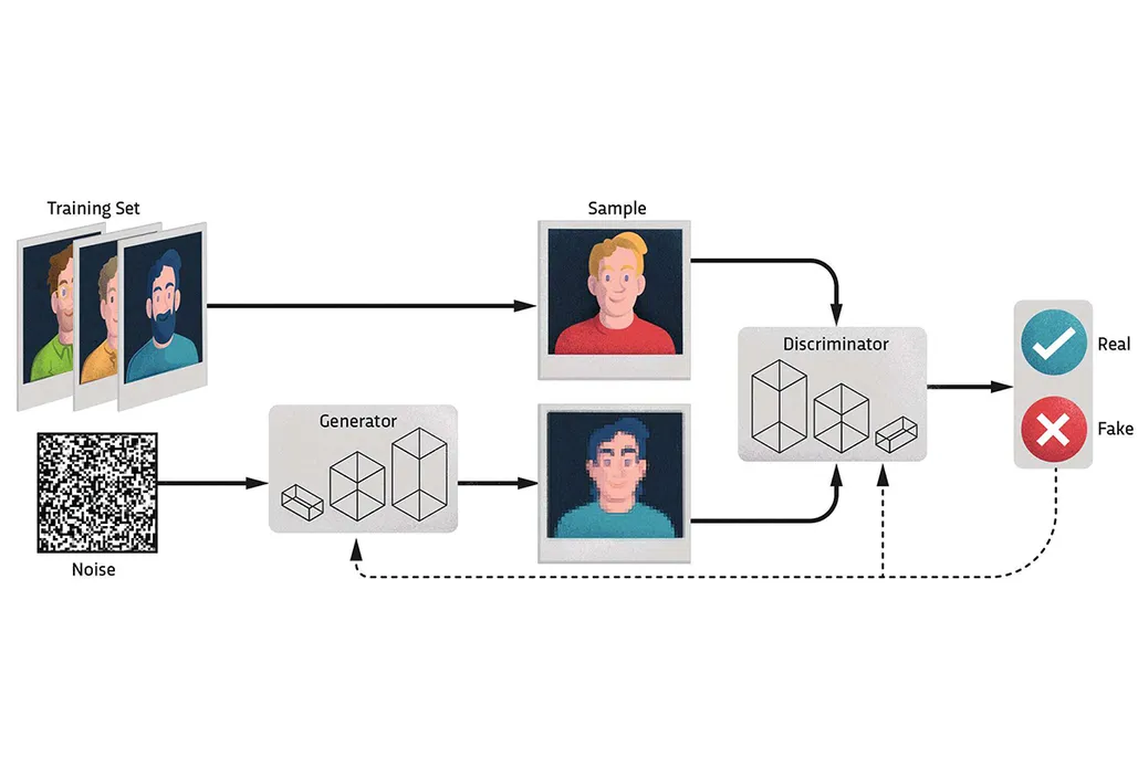
- GANs can generate realistic-looking images, text, or audio by learning the underlying distribution of the dataset.
- Example: GAN-generated human faces (thispersondoesnotexist.com).
Example GAN code using PyTorch:
import torch.nn as nn import torch.optim as optim class Generator(nn.Module): def __init__(self): super(Generator, self).__init__() self.fc = nn.Linear(100, 784) # 100-d noise vector to 28x28 image def forward(self, x): return torch.tanh(self.fc(x)) generator = Generator() noise = torch.randn(1, 100) fake_image = generator(noise) -
Bootstrapping
- A statistical method that resamples data with replacement to create new samples.
- Useful in small datasets to increase training size.
- Often used in ensemble learning (e.g., bagging).
-
Synthetic Minority Over-sampling (SMOTE)
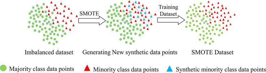
- Used in imbalanced datasets to generate synthetic minority class examples.
- Creates interpolated samples between existing data points.
- Example using
imbalanced-learn:
from imblearn.over_sampling import SMOTE from sklearn.model_selection import train_test_split X_resampled, y_resampled = SMOTE().fit_resample(X_train, y_train) -
Simulation-Based Synthesis
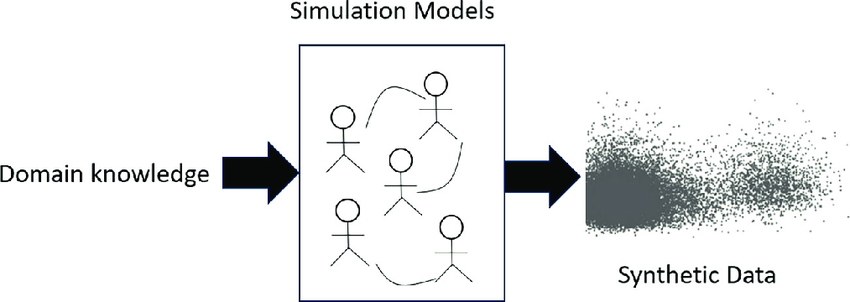
- Used in robotics, healthcare, and autonomous driving where real-world data collection is expensive or dangerous.
- Example: Self-driving cars trained on simulated environments before real-world deployment.
When to Use Data Augmentation vs. Data Synthesis?
| Method | Best for | Common Use Cases |
|---|---|---|
| Data Augmentation | Expanding existing datasets | Image classification, speech recognition |
| Data Synthesis | Creating new synthetic samples | GANs for image generation, NLP text synthesis |
Transfer Learning: Using Data from a Different Task
Transfer learning leverages pre-trained models:
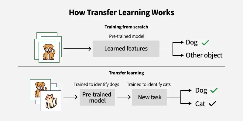
- Feature extraction: Use pre-trained model layers as feature extractors.
- Fine-tuning: Unfreeze layers and retrain on a new dataset.
Example: Using ImageNet-trained models for medical image classification.
Error Metrics for Skewed Datasets
In imbalanced datasets, accuracy alone is often misleading. For example, if a dataset has 95% negative samples and 5% positive samples, a model that always predicts “negative” will have 95% accuracy but is completely useless. Instead, we use more informative metrics:
Precision, Recall, and F1-Score
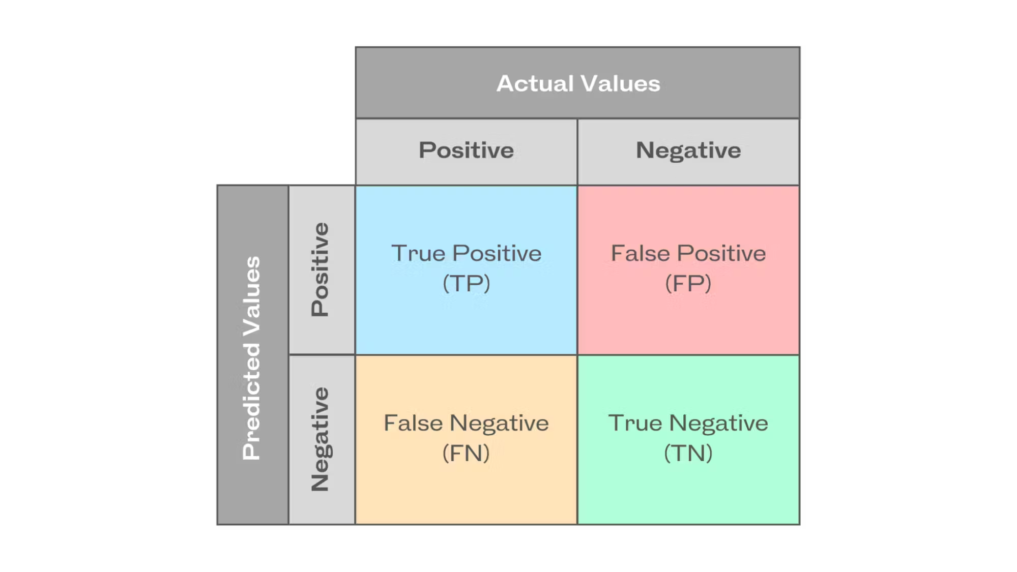
-
Precision ($P$): Measures how many of the predicted positives are actually correct.
$$ P = \frac{TP}{TP + FP} $$
- High Precision: The model makes fewer false positive errors.
- Example: In an email spam filter, high precision means fewer legitimate emails are mistakenly classified as spam.
-
Recall ($R$): Measures how many actual positives were correctly identified.
$$ R = \frac{TP}{TP + FN} $$
- High Recall: The model captures most of the actual positive cases.
- Example: In a medical test for cancer, high recall ensures that nearly all cancer cases are detected.
-
F1-Score: The harmonic mean of precision and recall, balancing both aspects.
$$ F_1 = 2 \times \frac{P \times R}{P + R} $$
- Used when both false positives and false negatives need to be minimized.
- F1-score ranges from 0 to 1, where 1 is the best possible score, indicating a perfect balance between precision and recall. However, what qualifies as a “good” or “bad” F1-score depends on the context of the problem.
Decision Trees
- Decision Tree Model
- Measuring Purity
- Choosing a Split: Information Gain
- Decision Trees for Continuous Features
- Regression Trees
- Using Multiple Decision Trees
Decision Tree Model
What is a Decision Tree?
A decision tree is a supervised machine learning algorithm used for classification and regression tasks. It mimics human decision-making by splitting data into branches based on feature values, forming a tree-like structure. The key components of a decision tree include:
- Root Node: The initial decision point that represents the entire dataset.
- Internal Nodes: Decision points where data is split based on a feature.
- Branches: The possible outcomes of a decision node.
- Leaf Nodes: The terminal nodes that provide the final classification or prediction.
graph TD;
    Root[Root Node] -->|Feature 1| Node1[Node 1];
    Root -->|Feature 2| Node2[Node 2];
    Node1 --> Leaf1[Leaf Node 1];
    Node1 --> Leaf2[Leaf Node 2];
    Node2 --> Leaf3[Leaf Node 3];
    Node2 --> Leaf4[Leaf Node 4];
Decision trees work by recursively splitting data based on a selected feature until a stopping condition is met.
Advantages and Disadvantages of Decision Trees
Advantages:
- Easy to Interpret: Decision trees provide an intuitive representation of decision-making.
- Handles Both Numerical and Categorical Data: They can work with mixed data types.
- No Need for Feature Scaling: Unlike algorithms like logistic regression or SVMs, decision trees do not require feature normalization.
- Works Well with Small Datasets: Decision trees can be effective even with limited data.
Disadvantages:
- Overfitting: Decision trees tend to learn patterns too specifically to the training data, leading to poor generalization.
- Sensitive to Noisy Data: Small variations in data can lead to different tree structures.
- Computational Complexity: For large datasets, training a deep tree can be time-consuming and memory-intensive.
Example: Classifying Fruits Using a Decision Tree
Consider a dataset containing different types of fruits characterized by their color, size, and texture. Our goal is to classify whether a given fruit is an apple or an orange.
| Color | Size | Texture | Fruit |
|---|---|---|---|
| Red | Small | Smooth | Apple |
| Green | Small | Smooth | Apple |
| Yellow | Large | Rough | Orange |
| Orange | Large | Rough | Orange |
Decision Tree Representation:
graph TD;
    Root[Is Size Large?]
    Root -- Yes --> Node1[Is Texture Rough?]
    Root -- No --> Apple[Apple]
    Node1 -- Yes --> Orange[Orange]
    Node1 -- No --> Apple[Apple]
The decision tree follows a top-down approach:
- The root node first checks whether the fruit is large.
- If yes, it checks whether the texture is rough.
- If the texture is rough, it classifies the fruit as an orange; otherwise, it’s an apple.
This example demonstrates how decision trees break down complex decision-making processes into simple binary decisions.
The learning process involves recursively splitting the dataset into smaller subsets. The splitting criterion is chosen based on purity measures such as Gini impurity or entropy. Each split creates child nodes until the stopping condition is met.
Stopping Criteria and Overfitting
A decision tree can continue growing until each leaf contains only one class. However, this often leads to overfitting, where the model memorizes the training data but fails to generalize to new data. To prevent this, stopping criteria such as:
- A minimum number of samples per leaf
- A maximum tree depth
- A minimum purity gain
can be used. Additionally, pruning techniques help reduce overfitting by removing branches that add little predictive value.
Pruning Example
- Pre-pruning: Stop the tree from growing beyond a certain depth.
- Post-pruning: Grow the full tree and then remove unimportant branches based on validation performance.
Measuring Purity
In decision trees, “purity” refers to how homogeneous the data in a given node is. A node is considered pure if it contains only samples from a single class. Measuring purity is essential for determining the best way to split a dataset to build an effective decision tree. The two most common metrics used for measuring purity are Entropy and Gini Impurity.
Entropy
Entropy, derived from information theory, measures the randomness or disorder in a dataset. The entropy equation for a binary classification problem is:
$$ H(S) = - p_1 \log_2(p_1) - p_2 \log_2(p_2) $$
where:
- $ p_1 $ and $ p_2 $ are the proportions of each class in the set $ S $.
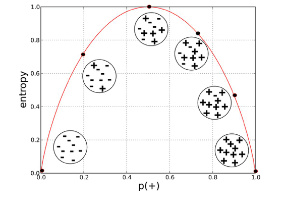
- Entropy = 0: The node is pure (all samples belong to one class).
- Entropy is high: The node contains a mix of different classes, meaning more disorder.
- Entropy is maximized at 0.5: If there is an equal probability of both classes (i.e., 50%-50%), the entropy is at its highest.
Example Calculation:
If a node contains 8 positive examples and 2 negative examples, the entropy is calculated as:
$$ H(S) = - \left( \frac{8}{10} \log_2 \frac{8}{10} + \frac{2}{10} \log_2 \frac{2}{10} \right) $$
$$ H(s) = 0.7958$$
Gini Impurity
Gini Impurity measures how often a randomly chosen element from the set would be incorrectly classified if it were randomly labeled according to the class distribution.
The formula for Gini impurity is:
$$ G(S) = 1 - \sum\limits_{i=1}^{C} p_i^2 $$
where:
- $ p_i $ is the probability of class $ i $ in the dataset.
graph TD;
    A(Class Distribution) -->|Pure Node| B(Entropy = 0, Gini = 0);
    A -->|50-50 Split| C(Entropy = 1, Gini = 0.5);
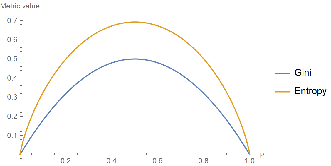
- Gini = 0: The node is completely pure.
- Gini is high: The node contains a mixture of classes.
Example Calculation:
For the same node with 8 positive and 2 negative examples:
$$ G(S) = 1 - \left( \left(\frac{8}{10}\right)^2 + \left(\frac{2}{10}\right)^2 \right) $$
$$ G(S) = 0.32 $$
Both metrics are used to determine the best way to split a node in a decision tree, but they have slight differences:
- Entropy is more computationally expensive since it involves logarithmic calculations.
- Gini Impurity is faster to compute and often preferred in decision tree implementations like CART (Classification and Regression Trees).
In practice, both perform similarly, and the choice depends on the specific problem and computational constraints.
By using these metrics, we can quantify the impurity of nodes and use them to decide the best possible splits while constructing a decision tree.
Choosing a Split: Information Gain
When constructing a decision tree, selecting the best feature to split on is crucial for building an optimal model. The goal is to maximize the Information Gain, which measures how well a feature separates the data into pure subsets.
Reducing Entropy
Information Gain (IG) is the reduction in entropy after splitting on a feature. It is calculated as:
$$ IG(S, A) = H(S) - \sum\limits_{v \in \text{Values}(A)} \frac{|S_v|}{|S|} H(S_v) $$
where:
- $ H(S) $ is the entropy of the original set.
- $ S_v $ represents subsets created by splitting on attribute $ A $.
- $ \frac{|S_v|}{|S|} $ is the weighted proportion of samples in each subset.
Example Calculation
Consider a dataset with the following samples:
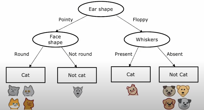
-
Compute initial entropy:
- 5
Catlabels and 5Doglabels.
-
$ p_1 = \frac{5}{10} $, $ \quad p_2 = \frac{5}{10} $.
-
$ H(S) = - \frac{5}{10} \log_2\frac{5}{10} - \frac{5}{10} \log_2\frac{5}{10} = 1.0 $.
- 5
-
Compute entropy after splitting by
Ear Shape:-
Subset
Pointy: {Cat, Cat, Cat, Cat, Dog}- $ H = -\frac{4}{5} \log_2\frac{4}{5} - \frac{1}{5} \log_2\frac{1}{5} \approx 0.72 $
-
Subset
Floppy: {Cat, Dog, Dog, Dog, Dog}- $ H = -\frac{1}{5} \log_2\frac{1}{5} - \frac{4}{5} \log_2\frac{4}{5} \approx 0.72 $
-
$ IG = 1.0 - (5/10)(0.72) - (5/10)(0.72) = 0.28 $
-
-
Compute entropy after splitting by
Face Shape:-
Subset
Round: {Cat, Cat, Cat, Dog, Dog, Dog, Cat}- $ H = -\frac{4}{7} \log_2\frac{4}{7} - \frac{3}{7} \log_2\frac{3}{7} \approx 0.99 $
-
Subset
Not Round: {Cat, Dog, Dog}- $ H = -\frac{1}{3} \log_2\frac{1}{3} - \frac{2}{3} \log_2\frac{2}{3} \approx 0.92 $
-
$ IG = 1.0 - (7/10)(0.99) - (3/10)(0.92) = 0.03 $
-
-
Compute entropy after splitting by
Whiskers:-
Subset
Present: {Cat, Cat, Cat, Dog}- $ H = -\frac{3}{4} \log_2\frac{3}{4} - \frac{1}{4} \log_2\frac{1}{4} \approx 0.81 $
-
Subset
Absent: {Dog, Dog, Dog, Dog, Cat, Cat}- $ H = -\frac{4}{6} \log_2\frac{4}{6} - \frac{2}{6} \log_2\frac{2}{6} \approx 0.92 $
-
$ IG = 1.0 - (4/10)(0.81) - (6/10)(0.92) = 0.12 $
-
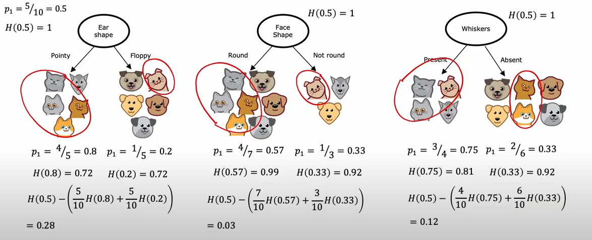
Since the highest Information Gain is $0.28$ (Ear Shape), splitting on either of these features is optimal.
Decision Trees for Continuous Features
When working with continuous features, decision trees can still be used effectively to predict outcomes, just like with categorical features.
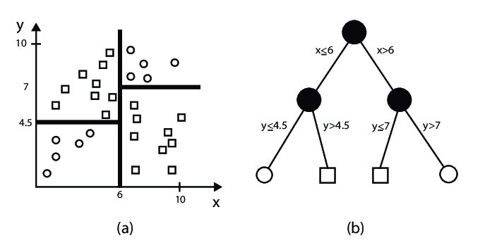
The key difference is that instead of using categorical values for splitting, decision trees for continuous features will determine optimal cutoffs or thresholds in the data. This allows the algorithm to make predictions for continuous target variables based on continuous input features.
In this example, we will predict whether an animal is a cat or dog based on its weight, using a decision tree that handles continuous features.
Let’s say we have the following dataset of animals, and we want to predict if the animal is a cat or dog based on its weight:
| Animal | Weight (kg) |
|---|---|
| Cat | 4.5 |
| Cat | 5.1 |
| Cat | 4.7 |
| Dog | 8.2 |
| Dog | 9.0 |
| Cat | 5.3 |
| Dog | 10.1 |
| Dog | 11.4 |
| Dog | 12.0 |
| Dog | 9.8 |
Here, we aim to build a decision tree based on the Weight feature to determine whether an animal is a cat or a dog.
Step 1: Find the Best Split for the Weight Feature
We will evaluate potential splits based on the Weight feature. The decision tree will consider possible cutoffs and calculate the impurity or variance for each split.
Let’s consider the following splits:
- Weight ≤ 7.0 kg: Assign
Cat - Weight > 7.0 kg: Assign
Dog
The decision tree will evaluate these splits by computing the impurity (for classification) or variance (for regression) for each possible split.
Step 2: Train a Decision Tree Model
We can use a decision tree to learn the best split and predict the animal type based on the weight. Here is how we can implement this in Python:
import numpy as np
from sklearn.tree import DecisionTreeClassifier
import pandas as pd

# Creating the dataset
data = {
    'Weight': [4.5, 5.1, 4.7, 8.2, 9.0, 5.3, 10.1, 11.4, 12.0, 9.8],
    'Animal': ['Cat', 'Cat', 'Cat', 'Dog', 'Dog', 'Cat', 'Dog', 'Dog', 'Dog', 'Dog']
}
df = pd.DataFrame(data)

# Splitting features and target
X = df[['Weight']]  # Feature
y = df['Animal']  # Target

# Training a decision tree classifier
clf = DecisionTreeClassifier(criterion='gini', max_depth=1)
clf.fit(X, y)

# Predicting animal type
predictions = clf.predict(X)
print(f'Predicted Animals: {predictions}')
Step 3: Visualizing the Decision Tree
The decision tree can be visualized to show how the split is made based on the Weight feature.
from sklearn.tree import plot_tree
import matplotlib.pyplot as plt

plt.figure(figsize=(10,8))
plot_tree(clf, feature_names=['Weight'], class_names=['Cat', 'Dog'], filled=True)
plt.show()
Step 4: Interpreting the Results
The resulting decision tree will have a root node where the Weight feature is split at a threshold (e.g., $7.0$ kg). If the animal’s weight is less than or equal to $7.0$ kg, it is classified as a Cat; otherwise, it is classified as a Dog.
Regression Trees
Regression trees are used when the target variable is continuous rather than categorical. Unlike classification trees, which predict discrete labels, regression trees predict numerical values by recursively partitioning the data and assigning an average value to each leaf node.
How Regression Trees Work
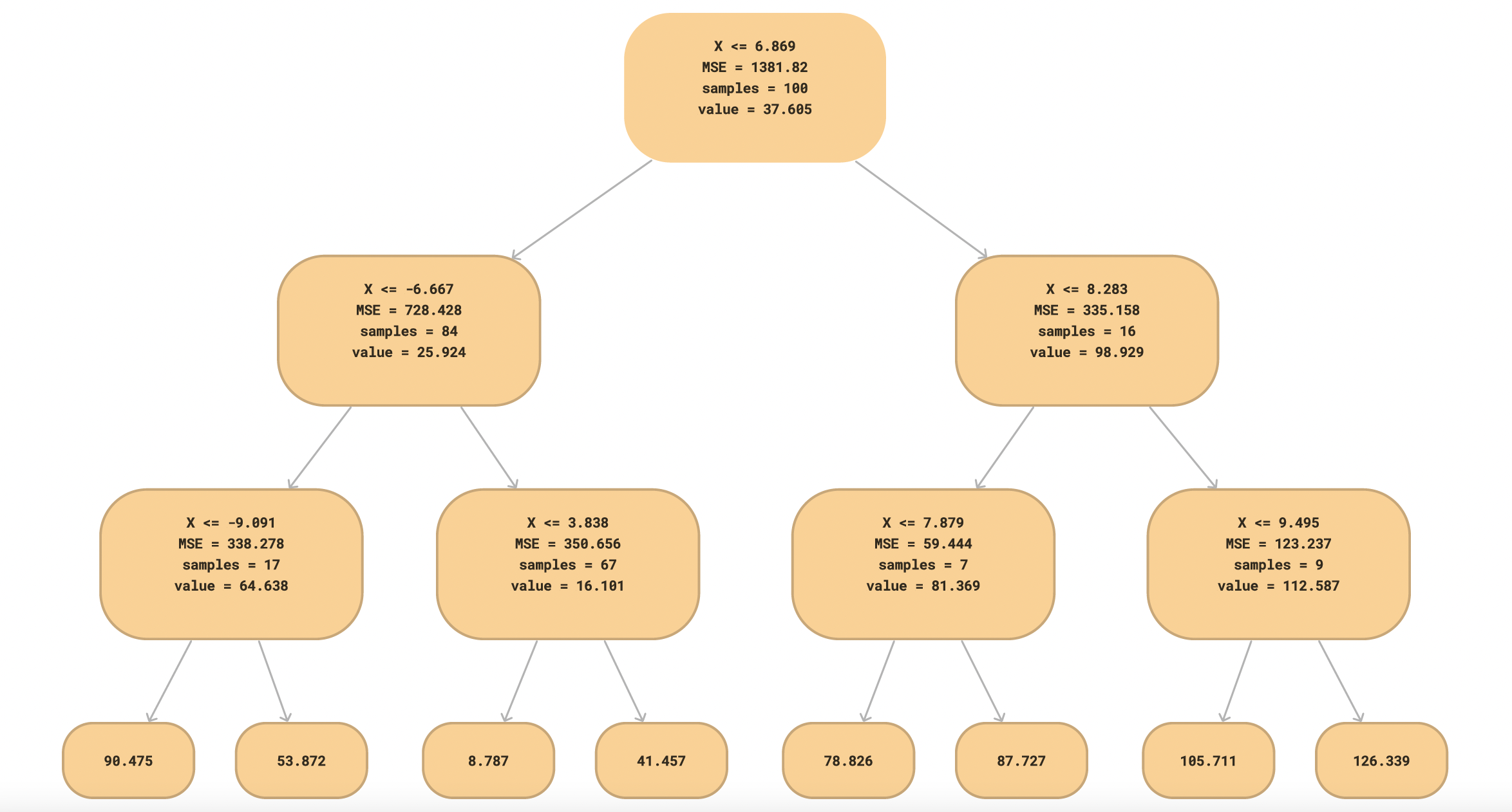
- Splitting the Data: The algorithm finds the best feature and threshold to split the data by minimizing variance.
- Assigning Values to Leaves: Instead of class labels, leaf nodes store the mean of the target values in that region.
- Prediction: Given a new sample, traverse the tree based on feature values and return the mean value from the corresponding leaf node.
Example: Predicting Animal Weights
We extend our dataset by adding a new feature: Weight. Our dataset consists of 10 animals, with the following features:
- Ear Shape: (Pointy, Floppy)
- Face Shape: (Round, Not Round)
- Whiskers: (Present, Absent)
- Weight (kg): Continuous target variable
| Ear Shape | Face Shape | Whiskers | Animal | Weight (kg) |
|---|---|---|---|---|
| Pointy | Round | Present | Cat | 4.5 |
| Pointy | Round | Present | Cat | 5.1 |
| Pointy | Round | Absent | Cat | 4.7 |
| Pointy | Not Round | Present | Dog | 8.2 |
| Pointy | Not Round | Absent | Dog | 9.0 |
| Floppy | Round | Present | Cat | 5.3 |
| Floppy | Round | Absent | Dog | 10.1 |
| Floppy | Not Round | Present | Dog | 11.4 |
| Floppy | Not Round | Absent | Dog | 12.0 |
| Floppy | Round | Absent | Dog | 9.8 |
Building a Regression Tree
We use Mean Squared Error (MSE) to determine the best split. The split that results in the lowest MSE is selected.
Step 1: Compute Initial MSE
The overall mean weight is:
$$ \bar{y} = \frac{4.5 + 5.1 + 4.7 + 8.2 + 9.0 + 5.3 + 10.1 + 11.4 + 12.0 + 9.8}{10} = 7.61 $$
MSE before splitting: $$ MSE = \frac{1}{10} \sum (y_i - \bar{y})^2 \approx 6.84 $$
Step 2: Find the Best Split
We evaluate splits based on feature values:
-
Split on Ear Shape:
- Pointy: ${(4.5, 5.1, 4.7, 8.2, 9.0)}$ → Mean = $6.3$
- Floppy: ${(5.3, 10.1, 11.4, 12.0, 9.8)}$ → Mean = $9.72$
- MSE = $3.2$ (better than initial MSE)
-
Split on Face Shape:
- Round: ${(4.5, 5.1, 4.7, 5.3, 10.1, 9.8)}$ → Mean = $6.58$
- Not Round: ${(8.2, 9.0, 11.4, 12.0)}$ → Mean = $10.15$
- MSE = $2.9$ (even better)
-
Split on Whiskers:
- Present: ${(4.5, 5.1, 8.2, 5.3, 11.4)}$ → Mean = $6.9$
- Absent: ${(4.7, 9.0, 10.1, 12.0, 9.8)}$ → Mean = $9.12$
- MSE = $3.1$ (better than initial but worse than Face Shape)
Thus, Face Shape is chosen as the first split.
Implementing in Python
import numpy as np
from sklearn.tree import DecisionTreeRegressor
import pandas as pd

# Creating the dataset
data = {
    'Ear_Shape': [0, 0, 0, 0, 0, 1, 1, 1, 1, 1],  # 0: Pointy, 1: Floppy
    'Face_Shape': [0, 0, 0, 1, 1, 0, 0, 1, 1, 0],  # 0: Round, 1: Not Round
    'Whiskers': [0, 0, 1, 0, 1, 0, 1, 1, 0, 0],  # 0: Present, 1: Absent
    'Weight': [4.5, 5.1, 4.7, 8.2, 9.0, 5.3, 10.1, 11.4, 12.0, 9.8]
}
df = pd.DataFrame(data)

# Splitting features and target
X = df[['Ear_Shape', 'Face_Shape', 'Whiskers']]
y = df['Weight']

# Training a regression tree
regressor = DecisionTreeRegressor(criterion='squared_error', max_depth=2)
regressor.fit(X, y)

# Predicting weights
predictions = regressor.predict(X)
print(f'Predicted Weights: {predictions}')
This regression tree provides predictions for the animal weights based on feature values.
Using Multiple Decision Trees
Using a single decision tree can sometimes lead to overfitting or instability, especially if the dataset has noise. By using multiple decision trees together, we can improve model performance and robustness. Two main techniques to achieve this are Bagging and Boosting.
Bagging (Bootstrap Aggregating)
Bagging reduces variance by training multiple decision trees on different random subsets of the dataset and then averaging their predictions. The most well-known example of bagging is the Random Forest algorithm.
Key Steps in Bagging:
- Draw random subsets (with replacement) from the training data.
- Train a decision tree on each subset.
- Combine predictions using majority voting (for classification) or averaging (for regression).
Visualization of Bagging:
graph TD;
    A[Dataset] -->|Bootstrap Sampling| B1[Tree 1];
    A[Dataset] -->|Bootstrap Sampling| B2[Tree 2];
    A[Dataset] -->|Bootstrap Sampling| B3[Tree 3];
    B1 --> C[Majority Vote];
    B2 --> C;
    B3 --> C;
Sampling with Replacement
Sampling with replacement is a technique where each data point has an equal probability of being selected multiple times in a new sample. This method is widely used in Bootstrap Aggregating (Bagging) to create multiple training datasets from the original dataset, allowing for robust model training and variance reduction.
- Why use Sampling with Replacement?
- It helps in reducing model variance.
- Generates multiple diverse datasets from the original dataset.
- Prevents overfitting by averaging multiple models.
Bootstrap Sampling Process
- Given a dataset of size $ N $, create a new dataset by randomly selecting $ N $ samples with replacement.
- Some original samples may appear multiple times, while others may not appear at all.
- Train multiple models on these sampled datasets and aggregate predictions.
Consider a dataset with five samples $ A, B, C, D, E $:
| Original Data | Bootstrap Sample 1 | Bootstrap Sample 2 |
|---|---|---|
| A | B | A |
| B | A | C |
| C | C | A |
| D | D | B |
| E | A | E |
Notice that in each bootstrap sample, some samples appear multiple times while others are missing.
Random Forest Algorithm
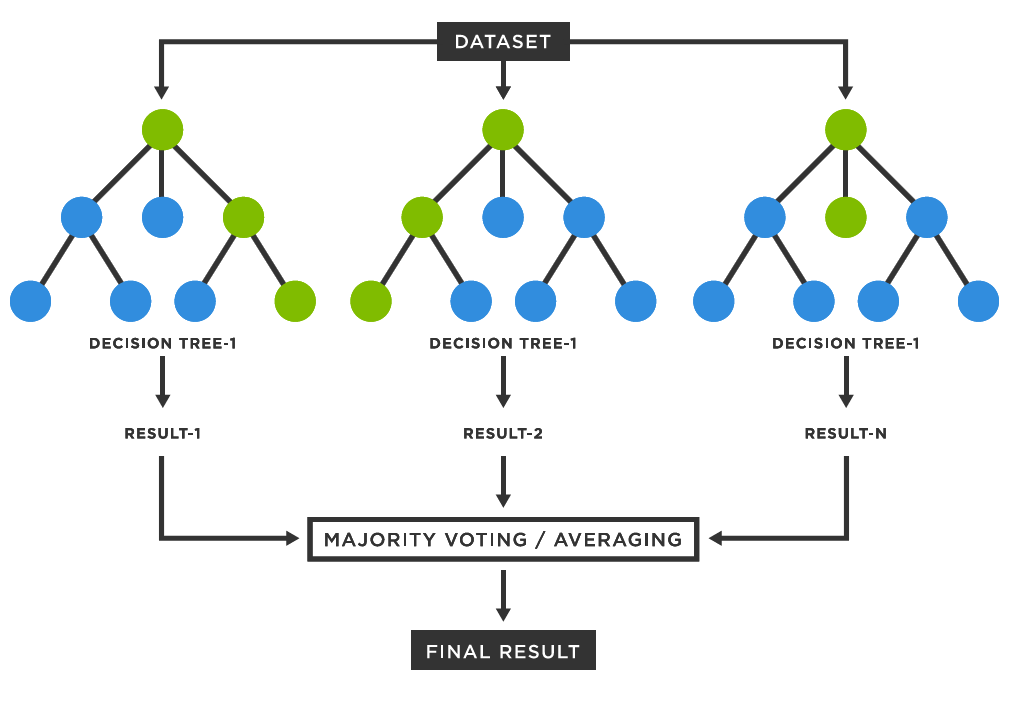
Random Forest is an ensemble learning method that builds multiple decision trees and merges them to achieve better performance. It is based on the concept of bagging (Bootstrap Aggregating), which helps reduce overfitting and improve accuracy.
How Random Forest Works
- Bootstrap Sampling: Randomly select subsets of the training data (with replacement).
- Decision Trees: Train multiple decision trees on different subsets.
- Feature Randomness: At each split, only a random subset of features is considered to introduce diversity.
- Aggregation:
- For classification, it takes a majority vote across all trees.
- For regression, it averages the predictions of all trees.
$$ Prediction_{RF} = \frac{1}{N} \sum_{i=1}^{N} Tree_i(x) $$
where $ N $ is the number of trees and $ Tree_i(x) $ is the prediction of the $ i^{th} $ tree.
Key Hyperparameters
| Hyperparameter | Description |
|---|---|
n_estimators | Number of decision trees in the forest |
max_depth | Maximum depth of each tree |
max_features | Number of features considered for splitting |
min_samples_split | Minimum samples required to split a node |
min_samples_leaf | Minimum samples required in a leaf node |
Decision Tree vs. Random Forest
graph TD;
    A[Dataset] -->|Training| B[Single Decision Tree];
    A -->|Bootstrap Sampling| C[Multiple Decision Trees];
    C -->|Aggregation| D[Final Prediction];
Random Forest example on Telco Customer Churn Dataset
import pandas as pd
import numpy as np
from sklearn.model_selection import train_test_split
from sklearn.ensemble import RandomForestClassifier
from sklearn.metrics import accuracy_score, classification_report

# Load the dataset
df = pd.read_csv('Telco-Customer-Churn.csv')

# Preprocessing
df = df.drop(columns=['customerID'])  # Remove non-relevant column
df = pd.get_dummies(df, drop_first=True)  # Convert categorical variables

# Splitting data
X = df.drop(columns=['Churn_Yes'])
y = df['Churn_Yes']
X_train, X_test, y_train, y_test = train_test_split(X, y, test_size=0.2, random_state=42)

# Train Random Forest model
rf = RandomForestClassifier(n_estimators=100, max_depth=10, random_state=42)
rf.fit(X_train, y_train)

# Predictions
y_pred = rf.predict(X_test)

# Evaluation
print("Accuracy:", accuracy_score(y_test, y_pred))
print(classification_report(y_test, y_pred))
When to Use Random Forest
- When you need high accuracy with minimal tuning.
- When dealing with large feature spaces.
- When feature importance is important.
- When you want to reduce overfitting compared to decision trees.
Random Forest is a powerful and flexible model that performs well across various datasets. However, it can be computationally expensive for large datasets.
Boosting
Boosting is another ensemble method that builds trees sequentially, with each tree trying to correct the mistakes of the previous one. It focuses on difficult examples by assigning them higher weights.
The most popular boosting method is XGBoost (Extreme Gradient Boosting).
Key Steps in Boosting:
- Train a weak model on the training data.
- Identify misclassified samples and assign them higher weights.
- Train the next model focusing on these hard cases.
- Repeat until a stopping criterion is met.
Visualization of Boosting:
graph TD;
    A[Dataset] -->|Train Weak Model| B1[Tree 1];
    B1 -->|Adjust Weights| B2[Tree 2];
    B2 -->|Adjust Weights| B3[Tree 3];
    B3 --> C[Final Prediction];
XGBoost
XGBoost (Extreme Gradient Boosting) is a powerful and efficient implementation of gradient boosting that is widely used in machine learning competitions and real-world applications due to its high performance and scalability.
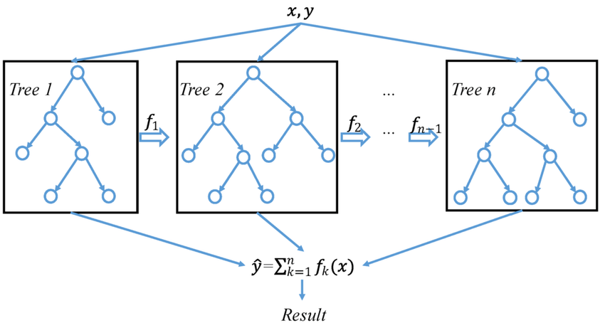
XGBoost builds an ensemble of decision trees sequentially, where each tree corrects the errors of the previous ones. The algorithm optimizes a loss function using gradient descent, allowing it to minimize errors effectively.
Key Components of XGBoost:
- Gradient Boosting Framework: Uses boosting to improve weak learners iteratively.
- Regularization: Includes L1 and L2 regularization to reduce overfitting.
- Parallelization: Optimized for fast training using parallel computing.
- Handling Missing Values: Automatically finds optimal splits for missing data.
- Tree Pruning: Uses depth-wise pruning instead of weight pruning for efficiency.
- Custom Objective Functions: Allows defining custom loss functions.
XGBoost optimizes the following objective function:
$$ J(\theta) = \sum L(y_i, \hat{y}_i) + \sum \Omega(T_k) $$
Where:
- $ L(y_i, \hat{y}_i) $ is the loss function (e.g., squared error for regression, log loss for classification).
- $ \Omega(T_k) $ is the regularization term controlling model complexity.
- $ T_k $ represents individual trees.
Implementing XGBoost on Telco Customer Churn Dataset
We will train an XGBoost model to predict customer churn.
Step 1: Load the dataset
import pandas as pd
from xgboost import XGBClassifier
from sklearn.model_selection import train_test_split
from sklearn.metrics import accuracy_score

# Load dataset
df = pd.read_csv("Telco-Customer-Churn.csv")

# Preprocess data
df = df.dropna()
df = pd.get_dummies(df, drop_first=True)

X = df.drop("Churn_Yes", axis=1)
y = df["Churn_Yes"]

# Split data
X_train, X_test, y_train, y_test = train_test_split(X, y, test_size=0.2, random_state=42)
Step 2: Train the XGBoost Model
xgb_model = XGBClassifier(n_estimators=100, learning_rate=0.1, max_depth=4, reg_lambda=1, use_label_encoder=False, eval_metric='logloss')
xgb_model.fit(X_train, y_train)
Step 3: Evaluate the Model
y_pred = xgb_model.predict(X_test)
accuracy = accuracy_score(y_test, y_pred)
print(f"Accuracy: {accuracy:.4f}")
Hyperparameter Tuning
Key hyperparameters in XGBoost:
| Hyperparameter | Description |
|---|---|
n_estimators | Number of trees in the model. |
learning_rate | Step size for updating weights. |
max_depth | Maximum depth of trees. |
subsample | Fraction of samples used per tree. |
colsample_bytree | Fraction of features used per tree. |
gamma | Minimum loss reduction required for split. |
When to Use XGBoost
- When you have structured/tabular data.
- When you need high accuracy.
- When you need a model that handles missing values efficiently.
- When feature interactions are important.
XGBoost is one of the most powerful algorithms for predictive modeling. By leveraging its strengths in handling structured data, regularization, and parallel processing, it can significantly outperform traditional machine learning methods in many real-world applications.
XGBoost vs Random Forest
| Feature | XGBoost | Random Forest |
|---|---|---|
| Training Speed | Faster (parallelized) | Slower |
| Overfitting Control | Stronger (Regularization) | Moderate |
| Performance on Structured Data | High | Good |
| Handles Missing Data | Yes | No |
K-means Clustering
- What is Clustering?
- K-Means Intuition
- K-Means Algorithm
- Optimization Objective
- Initializing K-Means
- Choosing the Number of Clusters
- Implementation of K-Means in Python
- Choosing the Number of Clusters
- Advantages and Disadvantages of K-Means
- Conclusion
What is Clustering?
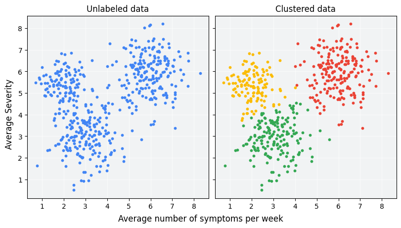
Clustering is an unsupervised learning technique used to group data points into distinct clusters based on their similarities. Unlike supervised learning, clustering does not rely on labeled data but instead identifies underlying structures within a dataset.
Applications of Clustering
- Customer Segmentation: Identifying groups of customers with similar purchasing behaviors.
- Anomaly Detection: Detecting fraudulent activities in financial transactions.
- Image Segmentation: Partitioning an image into meaningful regions.
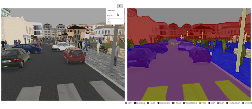
- Document Categorization: Grouping documents with similar topics.
- Genomics: Identifying gene expression patterns and categorizing biological data.
- Social Network Analysis: Detecting communities within a network.
K-Means Intuition
K-Means is one of the most widely used clustering algorithms due to its simplicity, efficiency, and scalability. The primary goal of K-Means is to partition a given dataset into K clusters by minimizing intra-cluster variance while maximizing inter-cluster differences.
Key Intuition:
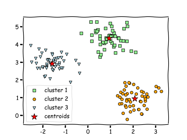
- Data points within the same cluster should be as similar as possible.
- Data points in different clusters should be as distinct as possible.
- The centroid of each cluster represents the
averageof all points in that cluster. - The algorithm iteratively improves the clusters until convergence.
K-Means Algorithm
The K-Means algorithm follows these steps:
- Initialize K cluster centroids randomly or using a specific method (e.g., K-Means++).
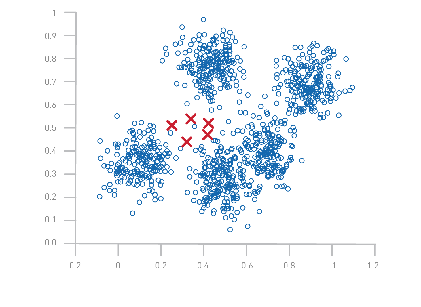
- Assign each data point to the nearest centroid using Euclidean distance:
$$
d(x, c) = \sqrt{(x_1 - c_1)^2 + (x_2 - c_2)^2 + \dots + (x_n - c_n)^2}
$$
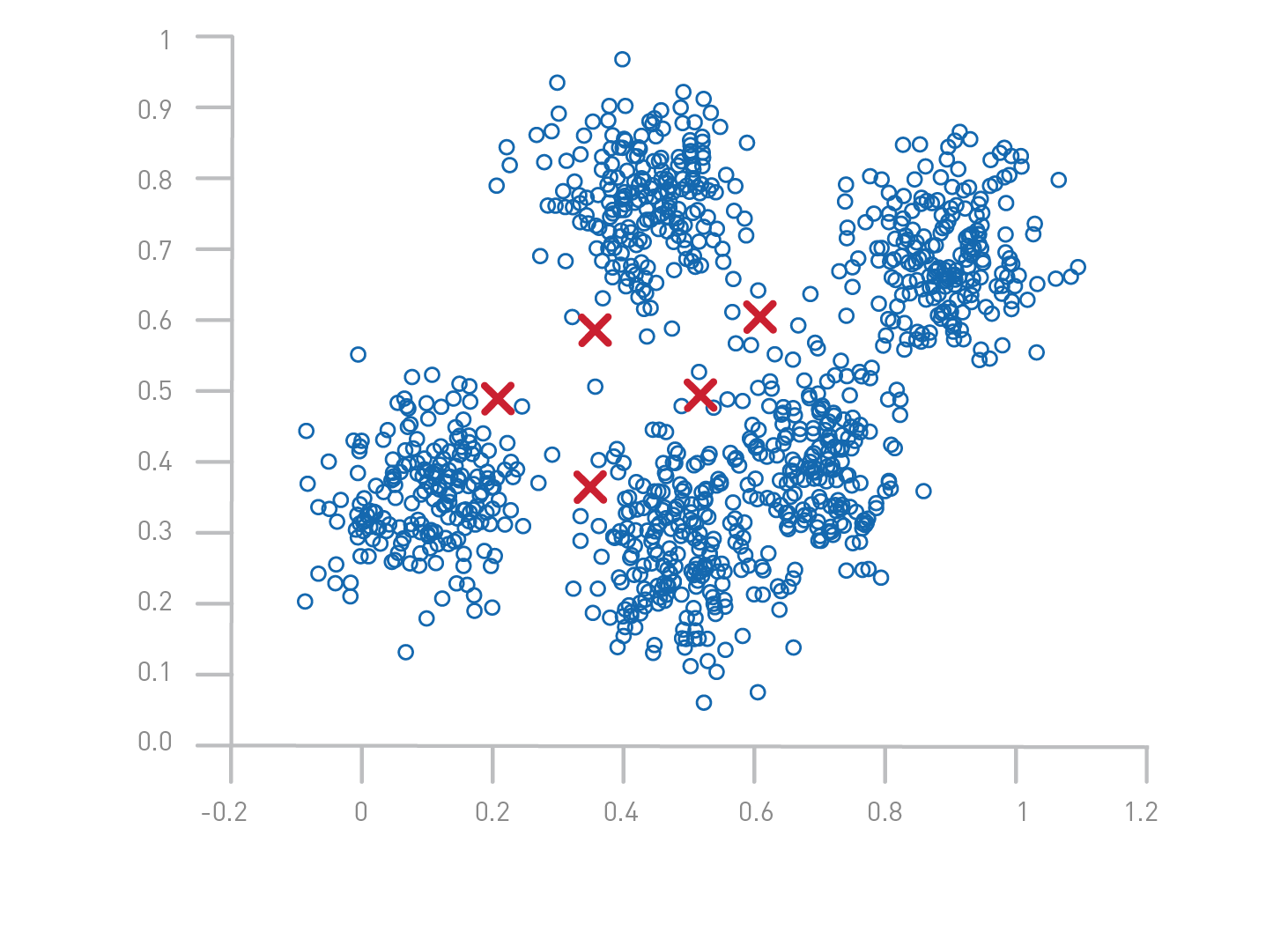
- Update centroids by computing the mean of all points assigned to each cluster:
$$
c_k = \frac{1}{N_k} \sum_{i=1}^{N_k} x_i
$$
where $ N_k $ is the number of points in cluster $ k $.
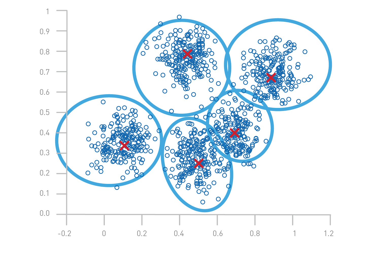
- Repeat until centroids stabilize (do not change significantly between iterations).
Optimization Objective
Consider data whose proximity measure is Euclidean distance. For our objective function, which measures the quality of a clustering, we use the sum of the squared error (SSE), which is also known as scatter.
In other words, we calculate the error of each data point, i.e., its Euclidean distance to the closest centroid, and then compute the total sum of the squared errors. Given two different sets of clusters that are produced by two different runs of K-means, we prefer the one with the smallest squared error, since this means that the prototypes (centroids) of this clustering are a better representation of the points in their cluster.
$$ J = \sum_{i=1}^{m} \sum_{k=1}^{K} w_{ik} ||x_i - c_k||^2 $$
where:
- $ x_i $ is a data point.
- $ c_k $ is the centroid of cluster $ k $.
- $ w_{ik} $ is 1 if $ x_i $ belongs to cluster $ k $, otherwise 0.
Initializing K-Means
Initialization significantly affects K-Means performance and results. Common initialization methods include:
- Random Initialization: Choosing K random points from the dataset.
- K-Means++ Initialization: A smarter method that spreads initial centroids to improve convergence speed and reduce the risk of poor clustering results.
- Forgy Method: Selecting K distinct data points as initial centroids.
Choosing the Number of Clusters
Selecting the appropriate number of clusters (K) is crucial. Common methods include:
- Elbow Method: Plotting WCSS vs. K and identifying the ‘elbow’ point.
- Silhouette Score: Measuring how similar a data point is to its own cluster vs. other clusters.
- Gap Statistic: Comparing WCSS against a random distribution to determine the optimal K.
Implementation of K-Means in Python
import numpy as np
import matplotlib.pyplot as plt
from sklearn.cluster import KMeans
from sklearn.datasets import make_blobs

# Create a synthetic dataset
X, _ = make_blobs(n_samples=300, centers=4, cluster_std=0.6, random_state=42)

# Apply K-Means
kmeans = KMeans(n_clusters=4, random_state=42)
kmeans.fit(X)
labels = kmeans.labels_
centroids = kmeans.cluster_centers_

# Plot the clusters
plt.scatter(X[:, 0], X[:, 1], c=labels, cmap='viridis', marker='o', edgecolor='black')
plt.scatter(centroids[:, 0], centroids[:, 1], s=200, c='red', marker='X')
plt.title("K-Means Clustering")
plt.show()
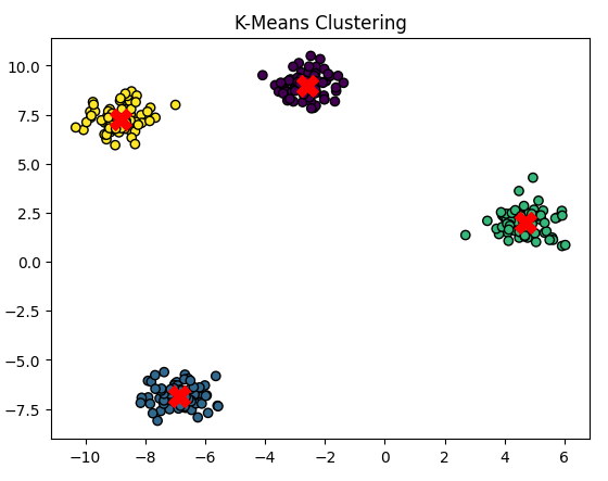
Choosing the Number of Clusters
Selecting the appropriate number of clusters (K) is crucial for obtaining meaningful results from K-Means clustering. Choosing too few clusters may result in underfitting, while choosing too many can lead to overfitting and unnecessary complexity. Several techniques help determine the optimal K:
1. Elbow Method
The Elbow Method is a widely used heuristic for selecting K by analyzing the Within-Cluster Sum of Squares (WCSS), also known as inertia.
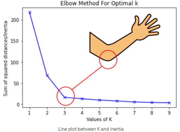
Steps:
- Run K-Means clustering for different values of K (e.g., from 1 to 10).
- Compute WCSS for each K. WCSS is defined as: $$ WCSS = \sum_{i=1}^{K} \sum_{x \in C_i} || x - \mu_i ||^2 $$ where $ \mu_i $ is the centroid of cluster $ C_i $ and $ x $ is a data point in that cluster.
- Plot WCSS vs. K and look for an ‘elbow’ point where the rate of decrease sharply changes.
- The optimal K is chosen at the elbow point, where adding more clusters does not significantly reduce WCSS.
2. Silhouette Score
The Silhouette Score measures how well-defined the clusters are by computing how similar a data point is to its own cluster compared to other clusters. It ranges from $-1$ to $1$:
- 1: Data point is well-clustered.
- 0: Data point is on the cluster boundary.
- -1: Data point is incorrectly clustered.
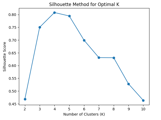
Steps:
- Compute the mean intra-cluster distance $ a(i) $ for each data point.
- Compute the mean nearest-cluster distance $ b(i) $ for each data point.
- Compute the silhouette score for each point: $$ S(i) = \frac{b(i) - a(i)}{\max(a(i), b(i))} $$
- The overall Silhouette Score is the average of all $ S(i) $.
- The optimal K is the one maximizing the Silhouette Score.
3. Gap Statistic
The Gap Statistic compares the clustering quality of the dataset against a random uniform distribution. It helps determine if a given clustering structure is significantly better than random clustering.
Steps:
- Run K-Means for different values of K and compute the within-cluster dispersion $ W_k $.
- Generate a random dataset with a similar range and compute $ W_k^{random} $.
- Compute the gap statistic: $$ G_k = \frac{1}{B} \sum_{b=1}^{B} \log(W_k^{random}) - \log(W_k) $$ where $ B $ is the number of random datasets.
- Choose the smallest K where $ G_k $ is significantly large.
Advantages and Disadvantages of K-Means
Advantages
- Simplicity: Easy to understand and implement.
- Scalability: Efficient for large datasets.
- Fast Convergence: Typically converges in a few iterations.
- Works well for convex clusters: If clusters are well-separated, K-Means performs effectively.
- Interpretable Results: Clusters can be easily visualized and analyzed.
Disadvantages
- Choice of K: Requires prior knowledge or heuristic methods to select the number of clusters.
- Sensitivity to Initialization: Poor initial centroid selection can lead to suboptimal results.
- Not Suitable for Non-Convex Shapes: Struggles with arbitrarily shaped clusters.
- Affected by Outliers: Outliers can skew centroids, leading to poor clustering.
- Equal Variance Assumption: Assumes clusters have similar variance, which may not always hold.
Example of Poor Performance: If the dataset contains clusters with varying densities or non-spherical shapes, K-Means may misclassify data points. Alternatives like DBSCAN or Gaussian Mixture Models (GMMs) may perform better in such cases.
Conclusion
K-Means is a powerful clustering technique widely used across industries. While it is simple and efficient, it has limitations such as sensitivity to initialization and difficulty handling non-convex clusters. However, by applying optimization techniques and careful selection of K, it remains a strong tool in unsupervised learning.
Anomaly Detection
- Finding Unusual Events
- Gaussian (Normal) Distribution
- Anomaly Detection Algorithm
- Developing and Evaluating an Anomaly Detection System
- 5. Anomaly Detection vs. Supervised Learning
- Choosing What Features to Use
- Full Python Example with TensorFlow
Finding Unusual Events
Anomaly detection is the process of identifying rare or unusual patterns in data that do not conform to expected behavior. These anomalies may indicate critical situations such as fraud detection, system failures, or rare events in various fields like healthcare and finance.
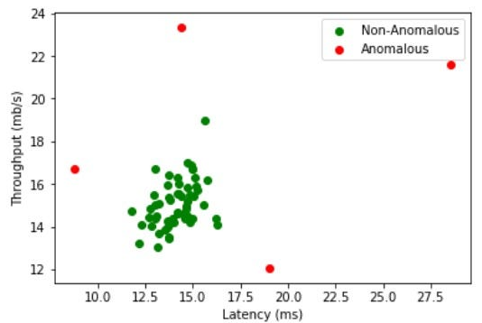
Real-World Examples
- Credit Card Fraud Detection: Identifying suspicious transactions that deviate significantly from a user’s normal spending habits.
- Manufacturing Defects: Detecting faulty products by identifying unusual patterns in production metrics.
- Network Intrusion Detection: Identifying cyber attacks by detecting unusual network traffic.
- Medical Diagnosis: Finding abnormal patterns in medical data that may indicate disease.
Gaussian (Normal) Distribution
The Gaussian distribution, also known as the normal distribution, is a fundamental probability distribution in statistics and machine learning. It is defined as:
$$ P(x) = \frac{1}{\sqrt{2 \pi \sigma^2}} e^{- \frac{(x - \mu)^2}{2 \sigma^2}} $$
Where:
- $ \mu $ is the mean (expected value)
- $ \sigma^2 $ is the variance
- $ x $ is the variable of interest
Properties of Gaussian Distribution
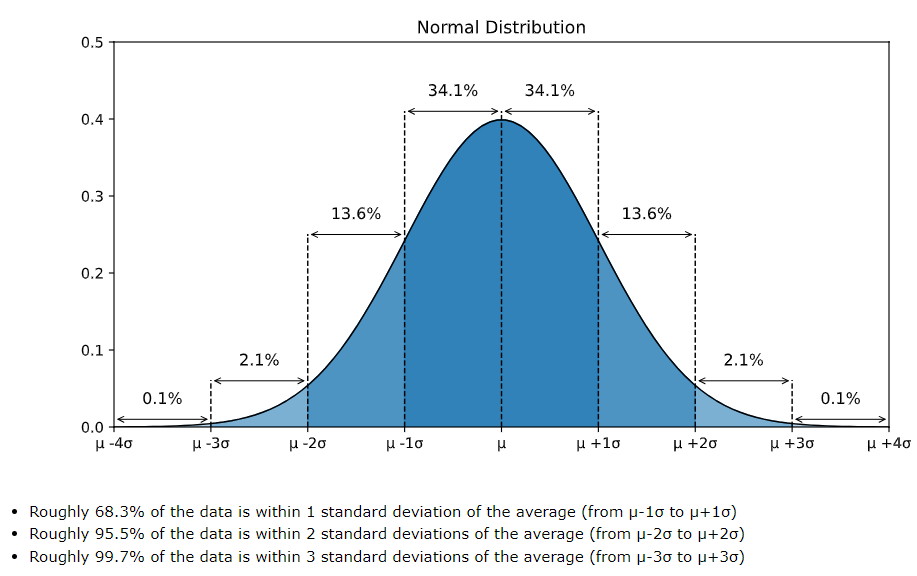
- Symmetric: Centered around the mean $ \mu $
- $68-95-99.7$ Rule:
- $68%$ of values lie within $1$ standard deviation ($ \sigma $) of the mean.
- $95%$ within $2$ standard deviations.
- $99.7%$ within $3$ standard deviations.
Gaussian distribution is often used in anomaly detection to model normal behavior, where deviations from this distribution indicate anomalies.
Anomaly Detection Algorithm
Steps in Anomaly Detection
- Feature Selection: Identify relevant features from the dataset.
- Model Normal Behavior: Fit a probability distribution (e.g., Gaussian) to the normal data.
- Calculate Probability Density: Use the learned distribution to compute the probability density of new data points.
- Set a Threshold: Define a threshold below which data points are classified as anomalies.
- Detect Anomalies: Compare new observations against the threshold.
Mathematical Approach
For a feature $ x $, assuming a Gaussian distribution:
$$
P(x) = \frac{1}{\sqrt{2 \pi \sigma^2}} e^{- \frac{(x - \mu)^2}{2 \sigma^2}}
$$
If $ P(x) $ is lower than a predefined threshold $ \epsilon $, then $ x $ is considered an anomaly:
$$
P(x) < \epsilon \Rightarrow x \text{ is an anomaly}
$$
Developing and Evaluating an Anomaly Detection System
Data Preparation
- Obtain a labeled dataset with normal and anomalous instances
- Preprocess data: Handle missing values, normalize features
Model Training
- Estimate parameters $ \mu $ and $ \sigma^2 $ using training data:
$$ \mu = \frac{1}{m} \sum\limits_{i=1}^{m} x^{(i)}, \quad \sigma^2 = \frac{1}{m} \sum\limits_{i=1}^{m} (x^{(i)} - \mu)^2 $$
- Compute probability density for test data
- Set anomaly threshold $ \epsilon $
Performance Evaluation
- Precision-Recall Tradeoff: Higher recall means catching more anomalies but may include false positives.
- F1 Score: Harmonic mean of precision and recall.
- ROC Curve: Evaluates different threshold settings.
5. Anomaly Detection vs. Supervised Learning
| Feature | Anomaly Detection | Supervised Learning |
|---|---|---|
| Labels Required? | No | Yes |
| Works with Unlabeled Data? | Yes | No |
| Suitable for Rare Events? | Yes | No |
| Examples | Fraud detection, Manufacturing defects | Spam detection, Image classification |
Choosing What Features to Use
- Domain Knowledge: Understand which features are relevant.
- Statistical Analysis: Use correlation matrices and distributions.
- Feature Scaling: Normalize or standardize data.
- Dimensionality Reduction: Use PCA or Autoencoders to reduce noise.
Full Python Example with TensorFlow
import numpy as np
import tensorflow as tf
from scipy.stats import norm
import matplotlib.pyplot as plt

# Generate synthetic normal data
np.random.seed(42)
data = np.random.normal(loc=50, scale=10, size=1000)

# Compute mean and variance
mu = np.mean(data)
sigma = np.std(data)

# Define probability density function
pdf = norm(mu, sigma).pdf(data)

# Set anomaly threshold (e.g., 0.001 percentile)
threshold = np.percentile(pdf, 1)

# Generate new test points
new_data = np.array([30, 50, 70, 100])
new_pdf = norm(mu, sigma).pdf(new_data)

# Detect anomalies
anomalies = new_data[new_pdf < threshold]
print("Anomalies detected:", anomalies)

# Plot
plt.figure(figsize=(10, 6))
plt.hist(data, bins=30, density=True, alpha=0.6, color='g')
x = np.linspace(min(data), max(data), 1000)
plt.plot(x, norm(mu, sigma).pdf(x), 'r', linewidth=2)
plt.scatter(anomalies, norm(mu, sigma).pdf(anomalies), color='red', marker='x', s=100, label='Anomalies')
plt.legend()
plt.show()
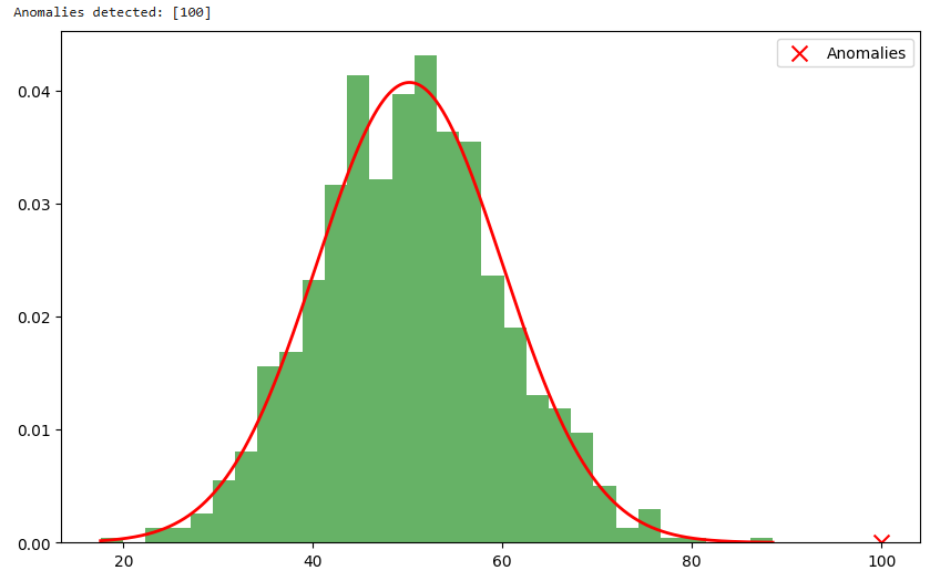
Explanation
- Generate synthetic data: We create a normal dataset.
- Compute mean and variance: Model normal behavior.
- Calculate probability density: Determine likelihood of each data point.
- Set threshold: Define an anomaly cutoff.
- Detect anomalies: Compare new observations against the threshold.
- Visualize results: Show normal distribution and detected anomalies.
This example provides a foundation for anomaly detection using probability distributions and can be extended with deep learning techniques like autoencoders or Gaussian Mixture Models (GMMs).
Recommender Systems
Recommender systems are everywhere in our digital lives, from Netflix suggesting movies based on our watch history to Amazon recommending products based on our previous purchases. These systems aim to predict what users might like based on their past behavior or the attributes of the items themselves.
Collaborative Filtering
Collaborative filtering is one of the most widely used techniques in recommender systems. It works by leveraging the behavior and preferences of users to make predictions about what they might like. Instead of relying on the characteristics of items themselves, collaborative filtering focuses on the interactions between users and items.
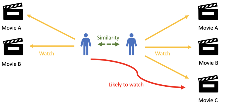
Imagine a streaming service like Netflix. If many users who watched “The Matrix” also watched “Inception,” the system might recommend “Inception” to a user who has already watched “The Matrix.” This works because the system assumes that similar users have similar tastes.
There are two main types of collaborative filtering:
- User-based Collaborative Filtering: Recommendations are made by finding users with similar preferences.
- Item-based Collaborative Filtering: Recommendations are made by finding similar items based on user interactions.
User-based Collaborative Filtering
Consider a movie recommendation system with four users (A, B, C, D) and seven movies (M1, M2, M3, M4, M5, M6, M7). The users have rated some of the movies on a scale from 1 to 5, but not every user has watched every movie. Our goal is to predict which unwatched movie user D would like the most and recommend it.
Below is the ratings matrix:
| User | M1 | M2 | M3 | M4 | M5 | M6 | M7 |
|---|---|---|---|---|---|---|---|
| A | 5 | 3 | 4 | - | 2 | - | 1 |
| B | 4 | - | 5 | 3 | 1 | 2 | - |
| C | 3 | 5 | - | 4 | - | 1 | 2 |
| D | - | 4 | 5 | 2 | 1 | - | - |
User D has not rated M1, M6, and M7, so we need to predict which one they are most likely to enjoy.
Finding Similar Users
We use a similarity measure to identify users most similar to D. A common choice is cosine similarity, defined as:
$$ \text{sim}(u, v) = \frac{ \sum_{i \in I} r_{ui} r_{vi} }{ \sqrt{ \sum_{i \in I} r_{ui}^2 } \sqrt{ \sum_{i \in I} r_{vi}^2 } } $$
where:
- $ r_{ui} $ is the rating of user $ u $ for item $ i $.
- $ I $ is the set of items rated by both users.
Computing similarity between D and other users:
Using cosine similarity, we compare D with other users:
| User | M2 | M3 | M5 |
|---|---|---|---|
| A | 3 | 4 | 2 |
| D | 4 | 5 | 1 |
$$ sim(D, A) = \frac{(4 \times 3) + (5 \times 4) + (1 \times 2)}{\sqrt{(4^2 + 5^2 + 1^2)} \times \sqrt{(3^2 + 4^2 + 2^2)}} = 0.974 $$
Similarly, we compute:
| User | M3 | M4 | M5 |
|---|---|---|---|
| B | 5 | 3 | 1 |
| D | 5 | 2 | 1 |
| User | M2 | M4 |
|---|---|---|
| C | 5 | 4 |
| D | 4 | 2 |
$$ sim(D, B) = 0.988, \quad sim(D, C) = 0.979 $$
Since B is most similar to D, we estimate D’s ratings for the unwatched movies (M1, M6, M7) using a weighted average:
$$ \hat{r}{D, j} = \bar{r}D + \frac{ \sum{u} , ext{sim}(D, u) \cdot (r{u, j} - \bar{r}u) }{ \sum{u} | ext{sim}(D, u)| } $$
Predicting Rating for M1
Using the weighted sum formula:
$$ \hat{r}{D, M1} = \frac{(sim(D, A) \times r{A, M1}) + (sim(D, B) \times r*{B, M1}) + (sim(D, C) \times r*{C, M1})}{sim(D, A) + sim(D, B) + sim(D, C)} $$
$$ \hat{r}_{D, M1} = \frac{(0.974 \times 5) + (0.988 \times 4) + (0.979 \times 3)}{0.974 + 0.988 + 0.979} = 3.998 $$
Repeating for M6 and M7, we get:
$$ \hat{r}{D, M6} = 1.494, \quad \hat{r}{D, M7} = 1.505 $$
Since M1 has the highest predicted rating (3.998), we recommend M1 to user D.
- Predicted rating for M1: 3.998
- Predicted rating for M6: 1.494
- Predicted rating for M7: 1.505
Since M1 has the highest predicted rating, we recommend M1 to D.
Item-based Collaborative Filtering
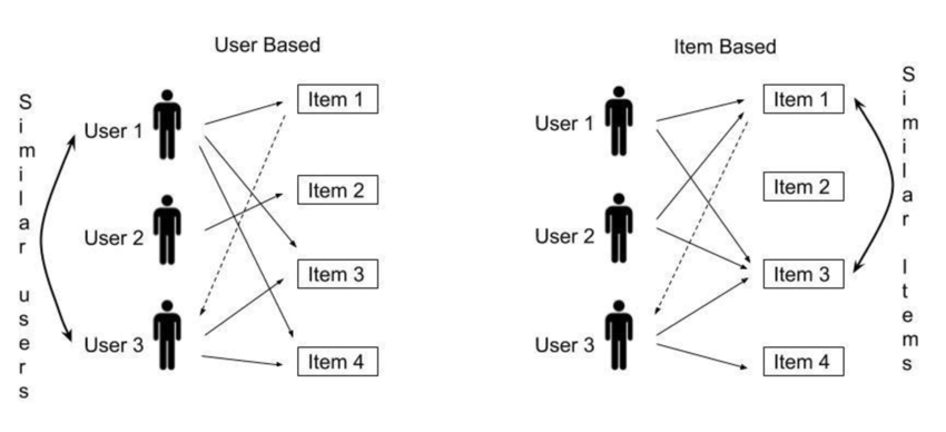
Rather than finding similar users, item-based collaborative filtering identifies similar items based on how users have rated them. The main idea is that if two movies are rated similarly by multiple users, they are likely to be similar.
Finding Similar Items
To determine item similarity, we use cosine similarity but compute it between movie rating vectors instead of user rating vectors.
Computing similarity between M1, M6, and M7 and other movies:
- sim(M1, M3) = 0.82
- sim(M6, M2) = 0.78
- sim(M7, M5) = 0.73
Since M3 is most similar to M1, we predict D’s rating for M1 based on D’s rating for M3:
$$ \hat{r}{D, M1} = \frac{ \sum{i} , ext{sim}(M1, i) \cdot r_{D, i} }{ \sum_{i} | ext{sim}(M1, i)| } $$
After calculations:
- Predicted rating for M1: 4.1
- Predicted rating for M6: 3.7
- Predicted rating for M7: 3.6
Since M1 has the highest predicted rating, we again recommend M1 to D.
Conclusion
- User-based filtering finds similar users and recommends based on their preferences.
- Item-based filtering finds similar items and predicts ratings based on a user’s history.
- Both methods predicted that D would like M1 the most, making it the best recommendation.
- These techniques can be combined for hybrid recommender systems to improve accuracy.
Content-Based Filtering
Content-based filtering recommends items to users by analyzing the characteristics of items a user has interacted with and comparing them with the characteristics of other items. Unlike collaborative filtering, which relies on user-item interactions, content-based filtering uses item metadata, such as genre, actors, or textual descriptions, to determine similarities.
Understanding Content-Based Filtering
In content-based filtering, each item is represented by a set of features. Users are assumed to have a preference for items with similar features to those they have previously liked. The recommendation process typically involves:
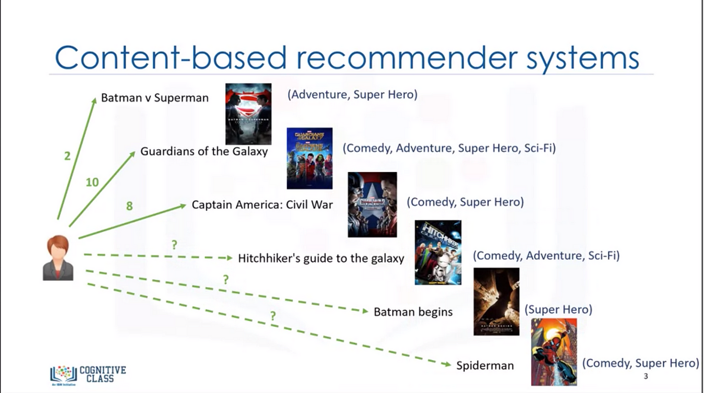
- Feature Representation: Representing items in terms of feature vectors.
- User Profile Construction: Creating a preference model for each user based on past interactions.
- Similarity Computation: Comparing new items with the user’s profile to generate recommendations.
- Generating Recommendations: Ranking items based on similarity scores and recommending the top ones.
To better understand this approach, let’s consider an example.
Example: Movie Recommendation
We have a dataset of seven movies, each described by three features: genre, director, and lead actor. Additionally, four users have rated some of these movies on a scale of 1 to 5.
Each movie is represented using a feature vector based on genre, director, and actors. We assign numerical values to categorical features using one-hot encoding.
| Movie | Action | Comedy | Drama | Sci-Fi | Director A | Director B | Actor X | Actor Y |
|---|---|---|---|---|---|---|---|---|
| M1 | 1 | 0 | 0 | 1 | 1 | 0 | 1 | 0 |
| M2 | 0 | 1 | 1 | 0 | 0 | 1 | 0 | 1 |
| M3 | 1 | 1 | 0 | 0 | 1 | 0 | 1 | 0 |
| M4 | 0 | 0 | 1 | 1 | 0 | 1 | 0 | 1 |
| M5 | 1 | 0 | 1 | 0 | 1 | 0 | 1 | 0 |
| M6 | 0 | 1 | 0 | 1 | 0 | 1 | 0 | 1 |
| M7 | 1 | 0 | 1 | 0 | 1 | 0 | 1 | 0 |
User Ratings
| User | M1 | M2 | M3 | M4 | M5 | M6 | M7 |
|---|---|---|---|---|---|---|---|
| A | 5 | 3 | 4 | - | 2 | - | 1 |
| B | 4 | - | 5 | 3 | 1 | 2 | - |
| C | 3 | 5 | - | 4 | - | 1 | 2 |
| D | - | 4 | 5 | 2 | 1 | - | - |
Step 1: Constructing User Profiles
For each user, we compute a preference vector by averaging the feature vectors of the movies they have rated, weighted by their ratings.
For example, user D has rated three movies: M2 (4), M3 (5), and M4 (2). Their profile vector is computed as:
$$ PD = \frac{4 \times V{M2} + 5 \times V*{M3} + 2 \times V*{M4}}{4 + 5 + 2} $$
This results in a vector representing user D’s preferences.
Step 2: Computing Similarity Scores
To recommend a new movie (e.g., M6 or M7), we compute the cosine similarity between the user’s preference vector and the feature vector of the candidate movies:
$$ \text{sim}(PD, V{Mi}) = \frac{PD \cdot V{Mi}}{||PD|| \times ||V{Mi}||} $$
Where $ PD \cdot V{Mi} $ is the dot product and $ ||PD|| $ and $ ||V{Mi}|| $ are the magnitudes.
Step 3: Generating Recommendations
By ranking the movies based on their similarity scores with the user’s profile, we can recommend the highest-ranked movie. If M6 has a similarity of 0.85 and M7 has 0.75, we recommend M6.
Advantages and Challenges of Content-Based Filtering
Advantages:
- Personalized recommendations based on individual preferences.
- Does not suffer from the cold start problem for items.
- No need for extensive user interaction data.
Challenges:
- Requires well-defined item features.
- Struggles with the cold start problem for new users.
- Limited to recommending items similar to those already interacted with.
By integrating deep learning techniques, such as word embeddings and neural networks, content-based filtering can improve accuracy and extend recommendations beyond direct similarities.
Principal Components Analysis (PCA)
Principal Components Analysis (PCA) is a dimensionality reduction technique used in machine learning and statistics to transform a large set of correlated features into a smaller set of uncorrelated features called principal components. This helps in reducing the complexity of data while retaining most of its variability.
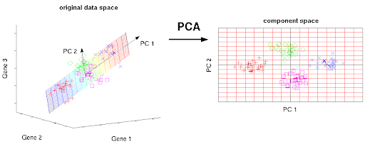
PCA is commonly used in:
- Reducing the number of features in high-dimensional datasets while preserving as much variance as possible.
- Visualizing high-dimensional data in 2D or 3D.
- Noise filtering and data compression.
- Feature extraction and selection.
Why PCA?
In many machine learning tasks, data often has a high number of dimensions, making computation expensive and difficult to interpret. For example, a movie recommender system might have thousands of features per movie (genre, director, actors, ratings, etc.). By using PCA, we can reduce this number to a smaller set of components that capture the most important patterns in the data.
How PCA Works
PCA involves the following steps:
- Standardization: The data is centered by subtracting the mean and scaled to have unit variance.
- Covariance Matrix Computation: A covariance matrix is computed to understand feature relationships.
- Eigenvalue and Eigenvector Computation: The eigenvalues and eigenvectors of the covariance matrix are found.
- Choosing Principal Components: The eigenvectors corresponding to the largest eigenvalues are selected as the principal components.
- Transforming the Data: The original data is projected onto the new principal component axes.
Mathematical Foundation of PCA
Step 1: Standardization
Since PCA relies on variance, the data should be standardized to have a mean of zero and unit variance:
$$ x’ = \frac{x - \mu}{\sigma} $$
where:
- $x$ is the original feature,
- $\mu$ is the mean of the feature,
- $\sigma$ is the standard deviation.
Step 2: Compute the Covariance Matrix
The covariance matrix captures relationships between different features:
$$ C = \frac{1}{n} X^T X $$
where $X$ is the standardized data matrix.
Step 3: Eigenvalues and Eigenvectors
PCA identifies principal components by computing eigenvalues and eigenvectors of the covariance matrix:
$$ C v = \lambda v $$
where:
- $\lambda$ are eigenvalues (variance captured by each principal component),
- $v$ are eigenvectors (principal component directions).
Step 4: Project Data onto Principal Components
Data is transformed into the new coordinate system:
$$ Z = X V_k $$
where $V_k$ contains the top $k$ eigenvectors.
PCA Visualization Example
We will visualize a dataset before and after applying PCA.
import numpy as np
import matplotlib.pyplot as plt
from sklearn.decomposition import PCA
from mpl_toolkits.mplot3d import Axes3D

# 3D veriyi oluşturma
np.random.seed(42)
n_samples = 100
mean1 = [2, 2, 2]
cov1 = [[1, 0.5, 0.2], [0.5, 1, 0.1], [0.2, 0.1, 1]]
data1 = np.random.multivariate_normal(mean1, cov1, n_samples)

mean2 = [5, 5, 5]
cov2 = [[1, -0.3, 0.1], [-0.3, 1, -0.2], [0.1, -0.2, 1]]
data2 = np.random.multivariate_normal(mean2, cov2, n_samples)

X = np.concatenate((data1, data2))
y = np.concatenate((np.zeros(n_samples), np.ones(n_samples)))

# 3D veriyi görselleştirme
fig = plt.figure(figsize=(12, 6))
ax = fig.add_subplot(121, projection='3d')
ax.scatter(X[:, 0], X[:, 1], X[:, 2], c=y, cmap='coolwarm', edgecolors='k')
ax.set_xlabel('X')
ax.set_ylabel('Y')
ax.set_zlabel('Z')
ax.set_title('Original 3D Data')

# PCA uygulama
pca = PCA(n_components=2)
X_pca = pca.fit_transform(X)

# 2D veriyi görselleştirme
ax2 = fig.add_subplot(122)
ax2.scatter(X_pca[:, 0], X_pca[:, 1], c=y, cmap='coolwarm', edgecolors='k')
ax2.set_xlabel('Principal Component 1')
ax2.set_ylabel('Principal Component 2')
ax2.set_title('Data After PCA (2D)')

plt.tight_layout()
plt.show()
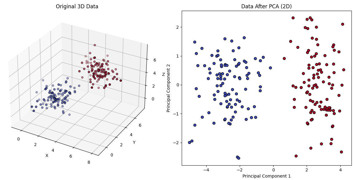
- The first plot shows the original dataset.
- The second plot shows the data projected onto the two principal components.
- PCA effectively captures the main variance in the data while reducing its dimensionality.
Conclusion
PCA is a fundamental technique for dimensionality reduction and data visualization. By identifying principal components, it helps uncover patterns, reduce noise, and improve machine learning model efficiency. However, PCA assumes linearity and may not perform well for highly non-linear data, where techniques like t-SNE or UMAP might be better alternatives.
Reinforcement Learning
- What is Reinforcement Learning?
- Markov Decision Process (MDP)
- State-Action Value Function ($Q(s,a)$)
- Bellman Equation
- Stochastic Environment (Randomness in RL)
- Continuous State vs. Discrete State
- Lunar Lander Example
- $ \varepsilon $-Greedy Policy
- Mini-Batch Learning in Reinforcement Learning
What is Reinforcement Learning?
Reinforcement Learning (RL) is a machine learning paradigm where an agent learns to make sequential decisions by interacting with an environment to maximize a cumulative reward. Unlike supervised learning, where labeled data is provided, RL relies on trial and error, receiving feedback in the form of rewards or penalties.
Key Characteristics of Reinforcement Learning:
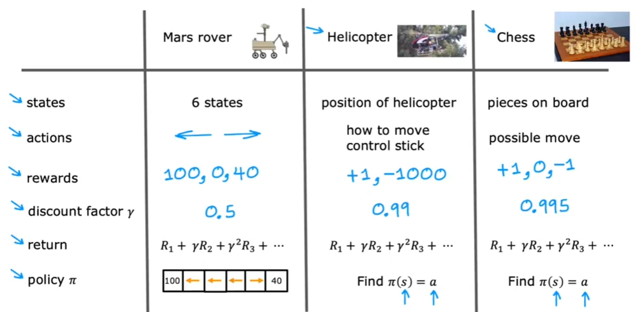
- Agent: The entity making decisions (e.g., a robot, a self-driving car, or an AI player in a game).
- Environment: The external system with which the agent interacts.
- State (s): A representation of the current situation of the agent in the environment.
- Action (a): A choice made by the agent at a given state.
- Reward (R): A numerical value given to the agent as feedback for its actions.
- Policy ( $ \pi$ ): A strategy that maps states to actions.
- Return (G): The cumulative reward collected over time.
- Discount Factor ( $ \gamma $ ): A value between 0 and 1 that determines the importance of future rewards.
Mars Rover Example
Let’s illustrate RL concepts using a Mars Rover example. Imagine a rover exploring a 1D terrain with six grid positions:
Each position is numbered from 1 to 6. The rover starts at position 4, and it can move left (-1) or right (+1). The goal is to maximize its rewards, which are given at positions 1 and 6:
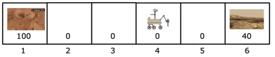
- Position 1 reward: 100 (e.g., a research station with supplies)
- Position 6 reward: 40 (e.g., a safe resting point)
- Other positions reward: 0
States, Actions, and Rewards
| State | Possible Actions | Reward |
|---|---|---|
| 1 | Move right (+1) | 100 |
| 2 | Move left (-1), Move right (+1) | 0 |
| 3 | Move left (-1), Move right (+1) | 0 |
| 4 (Start) | Move left (-1), Move right (+1) | 0 |
| 5 | Move left (-1), Move right (+1) | 0 |
| 6 | Move left (-1) | 40 |
- The agent (rover) must decide which direction to move.
- The state is the current position of the rover.
- The action is moving left or right.
- The reward depends on reaching the goal states (1 or 6).
How the Rover Decides Where to Go
The rover’s decision is based on maximizing its expected future rewards. Since it has two possible goal positions (1 and 6), it must evaluate different strategies. The rover should consider the following:
-
Immediate Reward Strategy
- If the rover focuses only on immediate rewards, it will move randomly, as most positions (except 1 and 6) have a reward of 0.
- This strategy is not optimal because it doesn’t take future rewards into account.
-
Short-Term Greedy Strategy
- If the rover chooses the nearest reward, it will likely go to position 6 since it’s closer than position 1.
- However, this might not be the best long-term decision.
-
Long-Term Reward Maximization
- The rover must evaluate how much discounted future reward it can accumulate.
- Even though position 6 has a reward of 40, position 1 has a much higher reward (100).
- If the rover can reliably reach position 1, it should favor this route, even if it takes more steps.
To formalize this, the rover can compute the expected return G for each possible path, considering the discount factor ($ \gamma $).
Discount Factor ($ \gamma $) and Expected Return
The discount factor $ \gamma $ determines how much future rewards are valued relative to immediate rewards. If $ \gamma = 1 $, all future rewards are considered equally important. If $ \gamma = 0.9 $, future rewards are slightly less important than immediate rewards.
For example, if the rover follows a path where it expects to reach position 1 in 3 steps and receive 100 reward, the discounted return is:
$$ G = 100 \times \gamma^3 = 100 \times 0.9^3 = 72.9 $$
If it reaches position 6 in 2 steps and receives 40 reward, the return is:
$$ G = 40 \times \gamma^2 = 40 \times 0.9^2 = 32.4 $$
Since 72.9 is greater than 32.4, the rover should prioritize going to position 1, even though it is farther away.
Policy ($ \pi $)
A policy ($ \pi $) defines the strategy of the rover: for each state, it dictates which action to take. Possible policies include:
- Greedy policy: Always moves towards the highest reward state immediately.
- Exploratory policy: Sometimes tries new actions to find better strategies.
- Discounted return policy: Balances short-term and long-term rewards.
If the rover follows an optimal policy, it should compute the total expected reward for every possible action and pick the one that maximizes its long-term return.
Markov Decision Process (MDP)
Reinforcement Learning problems are often modeled as Markov Decision Processes (MDPs), which are defined by:
- Set of States (S): $ s_1, s_2, …, s_n $
- Set of Actions (A): $ a_1, a_2, …, a_m $
- Transition Probability (P): Probability of moving from one state to another given an action $ P(s’ | s, a) $
- Reward Function (R): Defines the reward received when moving from $ s $ to $ s’ $
- Discount Factor ($ \gamma $): Determines the importance of future rewards.
In our Mars Rover example:
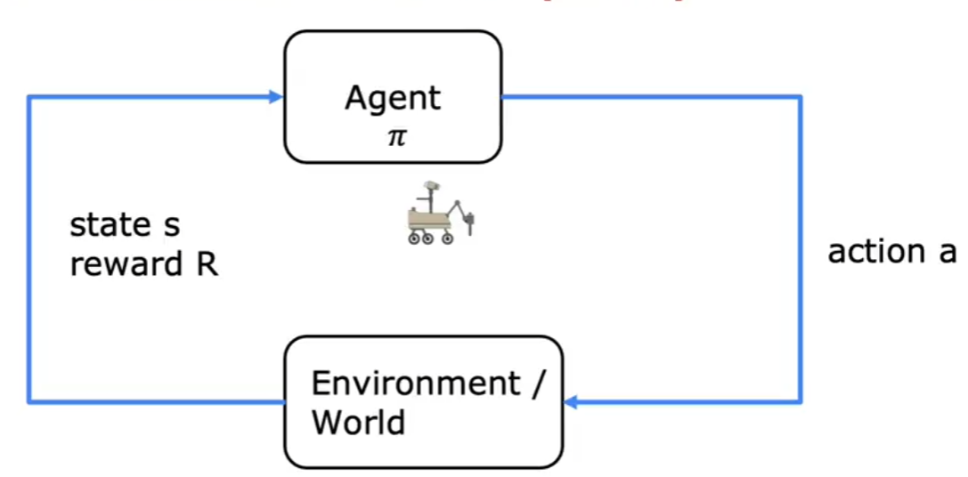
- States (S): {1, 2, 3, 4, 5, 6}
- Actions (A): {Left (-1), Right (+1)}
- Transition Probabilities (P): Deterministic (e.g., if the rover moves right, it always reaches the next state)
- Reward Function (R):
- $ R(1) = 100 $, $ R(6) = 40 $, $ R(2,3,4,5) = 0 $
- Discount Factor ($ \gamma $): $ 0.9 $ (assumed)
State-Action Value Function ($Q(s,a)$)
The State-Action Value Function, denoted as $Q(s,a)$, represents the expected return when starting from state $s$, taking action $a$, and then following a policy $\pi$. Formally:
$$ Q(s,a) = \mathbb{E} \big[ G_t \mid S_t = s, A_t = a \big] $$
This function helps the agent determine which action will lead to the highest reward in a given state.
Applying to Mars Rover
Using our Mars rover example, we can estimate $Q(s,a)$ values for each state-action pair. Suppose:
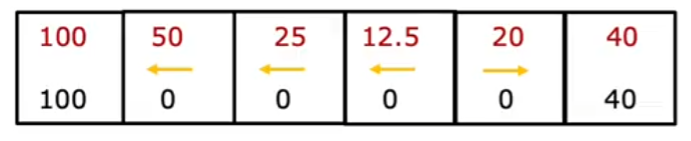
- $Q(4, \text{left}) = 25$
- $Q(4, \text{right}) = 20$
- $Q(5, \text{right}) = 40$
- $Q(3, \text{left}) = 50$
The rover should always select the action with the highest $Q$ value to maximize rewards.
Bellman Equation
The Bellman Equation provides a recursive relationship for computing value functions in reinforcement learning. It expresses the value of a state in terms of the values of successor states.
Understanding the Bellman Equation
In reinforcement learning, an agent makes decisions in a way that maximizes future rewards. However, since future rewards are uncertain, we need a way to estimate them efficiently. The Bellman equation helps us do this by breaking down the value of a state into two components:
- Immediate Reward ($R(s,a)$): The reward received by taking action $a$ in state $s$.
- Future Rewards ($V(s’)$): The expected value of the next state $s’$, weighted by the probability of reaching that state.
The Bellman equation is written as:
$$ V(s) = \max_a \Big[ R(s,a) + \gamma \sum_{s’} P(s’ | s,a) V(s’) \Big] $$
where:
- $V(s)$: The value of state $s$.
- $R(s,a)$: The immediate reward for taking action $a$ in state $s$.
- $\gamma$: The discount factor ($0 \leq \gamma \leq 1$), which determines how much future rewards are considered.
- $P(s’ | s,a)$: The probability of reaching state $s’$ after taking action $a$.
- $V(s’)$: The value of the next state $s’$.
Example Calculation for Mars Rover
Let’s assume:
- Moving from
4to3has a reward of-1. - Moving from
4to5has a reward of-1. - Position
1has a reward of100.
For $s=4$:
$$ V(4) = \max \big[ -1 + \gamma V(3), -1 + \gamma V(5) \big] $$
If we assume $V(3) = 50$ and $V(5) = 30$, and a discount factor $\gamma = 0.9$, we compute:
$$ V(4) = \max \big[ -1 + 0.9 \times 50, -1 + 0.9 \times 30 \big] $$
$$ V(4) = \max \big[ -1 + 45, -1 + 27 \big] $$
$$ V(4) = \max [44, 26] = 44 $$
Thus, the optimal value for state 4 is 44, meaning the agent should prefer moving left toward 3.
Intuition Behind the Bellman Equation
- The Bellman equation decomposes the value of a state into its immediate reward and the expected future reward.
- It allows us to compute values iteratively: we start with rough estimates and refine them over time.
- It helps in policy evaluation—determining how good a given policy is.
- It forms the foundation for Dynamic Programming methods like Value Iteration and Policy Iteration.
Stochastic Environment (Randomness in RL)
In real-world applications, environments are often stochastic, meaning actions do not always lead to the same outcome.
Stochasticity in the Mars Rover Example
Suppose the Mars rover’s motors sometimes malfunction, causing it to move in the opposite direction with a small probability (e.g., 10% of the time). Now, the transition dynamics include:
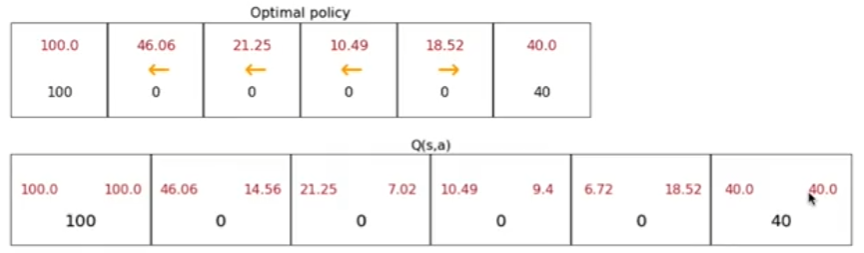
- $P(s’ = 5 | s = 4, a = \text{right}) = 0.9$
- $P(s’ = 3 | s = 4, a = \text{right}) = 0.1$
This randomness makes decision-making more challenging. Instead of just considering rewards, the rover must now account for expected rewards and the probability of ending up in different states.
Impact on Decision-Making
With stochastic environments, deterministic policies (always taking the best action) may not be optimal. Instead, an exploration-exploitation balance is needed:
- Exploitation: Following the best-known action based on past experience.
- Exploration: Trying new actions to discover potentially better rewards.
This concept is central to algorithms like Q-Learning and Policy Gradient Methods, which we will discuss in future sections.
Continuous State vs. Discrete State
In reinforcement learning, states can be either discrete or continuous. A discrete state means that the number of possible states is finite and well-defined, whereas a continuous state implies an infinite number of possible states.
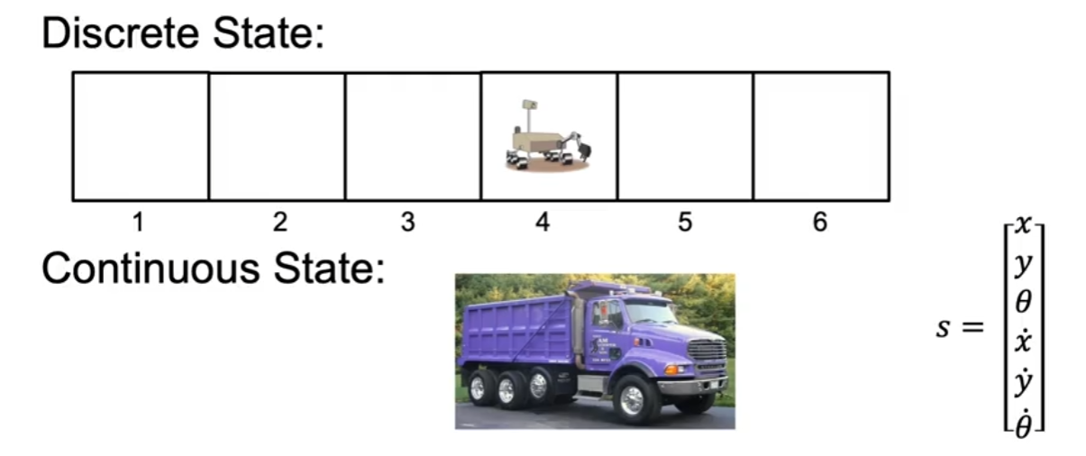
For example, consider our Mars Rover example with six possible states. The rover can be in any one of these six states at any given time, making it a discrete state environment. However, if we consider a truck driving on a highway, its position, speed, angle, and other attributes can take an infinite number of values, making it a continuous state environment.
Continuous state spaces are often approximated using function approximators like neural networks to generalize over an infinite number of states efficiently.
Lunar Lander Example
A classic reinforcement learning problem is the Lunar Lander, where the objective is to safely land a spacecraft on the surface of a planet. The agent (lander) interacts with the environment by selecting one of four possible actions:
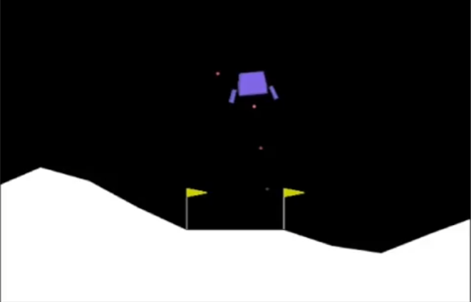
- Do Nothing: No thrust is applied.
- Left Thruster: Applies force to move left.
- Right Thruster: Applies force to move right.
- Main Thruster: Applies force to slow descent.
Rewards and Penalties:
The environment provides feedback through rewards and penalties:
- Soft Landing: +100 reward
- Crash Landing: -100 penalty
- Firing Main Engine: -0.3 penalty (fuel consumption)
- Firing Side Thrusters: -0.1 penalty (fuel consumption)
State Representation
The state of the lunar lander can be represented as:
$$ s = [x, y, \theta, l, r, x’, y’, \theta’] $$
where:
- $ x, y $ : Position of the lander
- $ \theta $ : Orientation (tilt angle)
- $ l, r $ : Contact with left and right landing pads (binary values)
- $ x’, y’ $ : Velocities in x and y directions
- $ \theta’ $ : Angular velocity
The policy function $ \pi(s) $ determines which action to take given the current state.
Deep Q-Network (DQN) Neural Network for Lunar Lander
To approximate the optimal policy, we use a deep neural network. The network takes the 8-dimensional state vector as input and predicts Q-values for each of the four actions.
Network Architecture:
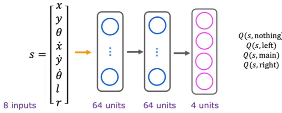
- Input Layer (8 neurons): Corresponds to $ x, y, \theta, l, r, x’, y’, \theta’ $
- Two Hidden Layers (64 neurons each, ReLU activation)
- Output Layer (4 neurons): Represents the Q-values for the four possible actions
The output neurons correspond to:
- $ Q(s, \text{do nothing}) $
- $ Q(s, \text{main thruster}) $
- $ Q(s, \text{right thruster}) $
- $ Q(s, \text{left thruster}) $
The network is trained using the Bellman equation to minimize the difference between predicted and actual Q-values.
$ \varepsilon $-Greedy Policy
In reinforcement learning, an agent must balance exploration (trying new actions) and exploitation (choosing the best-known action). The $ \varepsilon $-greedy policy is a common approach to achieve this balance:
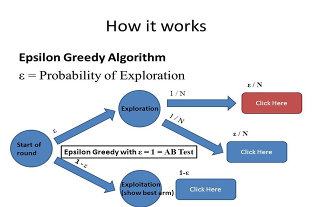
- With probability $ \varepsilon $, take a random action (exploration).
- With probability $ 1 - \varepsilon $, take the action with the highest Q-value (exploitation).
Initially, $ \varepsilon $ is set to a high value (e.g., 1.0) to encourage exploration and gradually decays over time.
Mini-Batch Learning in Reinforcement Learning
In deep reinforcement learning, we use mini-batch learning to improve training efficiency and stability.
Why Mini-Batch Learning?
- Prevents large updates from a single experience (stabilizes training).
- Helps break the correlation between consecutive experiences (improves generalization).
- Allows efficient GPU computation (faster convergence).
How It Works:
- Store experiences (state, action, reward, next state) in a replay buffer.
- Sample a mini-batch of experiences.
- Compute target Q-values using the Bellman equation.
- Perform a gradient descent update on the Q-network.
Mini-batch learning makes reinforcement learning more robust and prevents overfitting to recent experiences.
Content
∴
I completed the Deep Learning Specialization by taking detailed notes and summarizing critical concepts for future reference.
Stanford University & DeepLearning.AI
— emreaslan —
Computer Vision and Edge Detection
- Computer Vision
- Edge Detection
Computer Vision
Introduction to Computer Vision
Computer Vision is a field of artificial intelligence (AI) that enables machines to interpret and understand visual information from the world. It encompasses tasks such as image recognition, object detection, and segmentation.
Real-World Applications
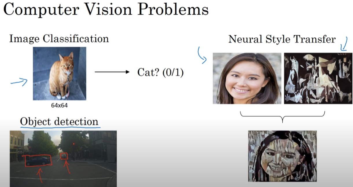
- Facial Recognition: Used in security systems and social media tagging.
- Medical Imaging: Helps in detecting diseases using X-rays, MRIs, and CT scans.
- Autonomous Vehicles: Enables self-driving cars to recognize objects and road signs.
- Industrial Automation: Used for defect detection in manufacturing.
Fundamental Concepts
- Pixels: The smallest unit in an image.
- Grayscale and Color Images: Difference between single-channel and multi-channel images.
- Resolution: Number of pixels in an image.
- Image Representation: Images as matrices of pixel values.
Mathematical Formulation
An image can be represented as a matrix:
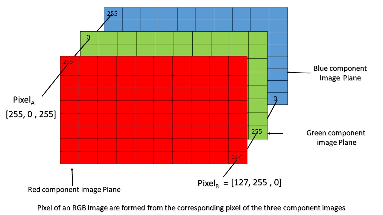
$$ I(x, y) \in \mathbb{R}^{m \times n \times c} $$
where $m$ and $n$ represent height and width, and $c$ represents the number of color channels (1 for grayscale, 3 for RGB images).
Edge Detection
Why Use Convolution for Edge Detection?
Edge detection aims to find points in an image where the intensity changes sharply. These points often correspond to boundaries of objects, texture changes, or discontinuities in depth. To detect these changes, we apply convolution operations with specific filters.
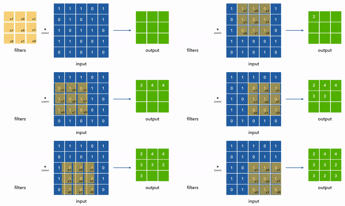
Convolution is a mathematical operation that helps us apply a small matrix (called a filter or kernel) across the entire image to detect specific patterns like edges.
What Does a Filter Do?
A filter is essentially a small grid of numbers (e.g., $3x3$) that slides across the image and emphasizes certain features:
- Edge filters highlight intensity changes
- Blur filters smooth the image
- Sharpening filters enhance details
In edge detection, filters are designed to detect high spatial frequency changes—essentially, edges.
Mathematical Example
$$ I = \left[ \begin{array}{cccccc} 12 & 15 & 14 & 10 & 9 & 10 \ 18 & 20 & 22 & 17 & 14 & 12 \ 24 & 28 & 30 & 26 & 20 & 18 \ 30 & 33 & 35 & 32 & 28 & 25 \ 22 & 25 & 28 & 24 & 22 & 20 \ 15 & 17 & 19 & 18 & 16 & 15 \end{array} \right] $$
We apply a vertical Sobel filter $ K_v $:
$$ K_v = \left[ \begin{array}{ccc} -1 & 0 & 1 \ -2 & 0 & 2 \ -1 & 0 & 1 \end{array} \right] $$
This filter detects vertical edges by highlighting horizontal intensity transitions.
Step-by-Step Convolution (No Padding, Stride = 1)
Let’s compute the top-left value of the output matrix. We place the filter on the top-left 3x3 window of ( I ):
Window:
$$ \left[ \begin{array}{ccc} 12 & 15 & 14 \ 18 & 20 & 22 \ 24 & 28 & 30 \end{array} \right] $$
Element-wise multiplication and sum:
$$ (-1 \cdot 12) + (0 \cdot 15) + (1 \cdot 14) + (-2 \cdot 18) + (0 \cdot 20) + (2 \cdot 22) + (-1 \cdot 24) + (0 \cdot 28) + (1 \cdot 30) $$
$$ = -12 + 0 + 14 - 36 + 0 + 44 - 24 + 0 + 30 = 16 $$
So, the top-left value of the output matrix is 16.
Second Convolution Step (Next to Right)
New window (move filter one step to the right):
$$ \left[ \begin{array}{ccc} 15 & 14 & 10 \ 20 & 22 & 17 \ 28 & 30 & 26 \end{array} \right] $$
Apply the same operation:
$$ (-1 \cdot 15) + (0 \cdot 14) + (1 \cdot 10) + (-2 \cdot 20) + (0 \cdot 22) + (2 \cdot 17) + (-1 \cdot 28) + (0 \cdot 30) + (1 \cdot 26) $$
$$ = -15 + 0 + 10 - 40 + 0 + 34 - 28 + 0 + 26 = -13 $$
So, second value is -13.
Full Output Matrix (4x4)
After sliding the filter across the 6x6 image, we get the 4x4 output:
$$ I * K_v = \left[ \begin{array}{cccc} 16 & -13 & -25 & -26 \ 20 & -11 & -22 & -24 \ 12 & -8 & -18 & -16 \ 4 & -5 & -9 & -8 \end{array} \right] $$
This matrix highlights the vertical edges in the original image—areas where pixel intensities change most dramatically from left to right.
The result of convolving the image with these filters gives us areas of strong gradient—edges.
Key Insight:
Filters translate the idea of change in pixel values into a computable quantity.
Edge Detection Techniques
1. Sobel Operator
- Combines Gaussian smoothing and differentiation.
- Horizontal ($ G_x $) and vertical ($ G_y $) gradients are calculated using predefined 3x3 kernels.
$$ 3 x 3 \text(Sobel Kernels)$$
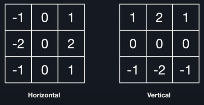
- The gradient magnitude is: $$ G = \sqrt{G_x^2 + G_y^2}, \quad \theta = \tan^{-1}\left(\frac{G_y}{G_x}\right) $$
- Commonly used due to simplicity and noise resistance.
- Watch this youtube video
2. Prewitt Operator
- Similar to Sobel, but with uniform weights.
$$ 3 x 3 \text(Prewitt Kernels)$$
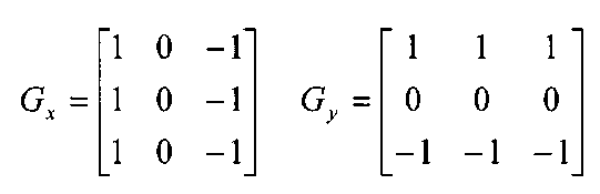
- Slightly less sensitive to noise compared to Sobel.
3. Laplacian of Gaussian (LoG)
- A second derivative method.
- Detects edges by identifying zero-crossings after applying the Laplacian to a Gaussian-smoothed image.
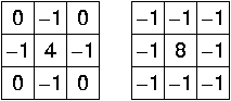
- Equation: $$ \nabla^2 I = \frac{\partial^2 I}{\partial x^2} + \frac{\partial^2 I}{\partial y^2} $$
- Sensitive to noise, hence Gaussian smoothing is applied first.
4. Canny Edge Detection
A multi-stage algorithm designed for optimal edge detection:
- Gaussian Filtering: Noise reduction.
- Gradient Calculation: Using Sobel filters.
- Non-Maximum Suppression: Thinning the edges.
- Double Thresholding: Classify edges as strong, weak, or non-edges.
- Hysteresis: Connect weak edges to strong ones if they are adjacent.
Canny is widely used in practice for its high accuracy and low false detection.
5. Difference of Gaussians (DoG)
- Approximates the LoG by subtracting two Gaussian-blurred images: $$ DoG = G_{\sigma_1} * I - G_{\sigma_2} * I $$
- Faster to compute than LoG.
- Used in blob detection and feature matching.
Convolutional Operations
Padding
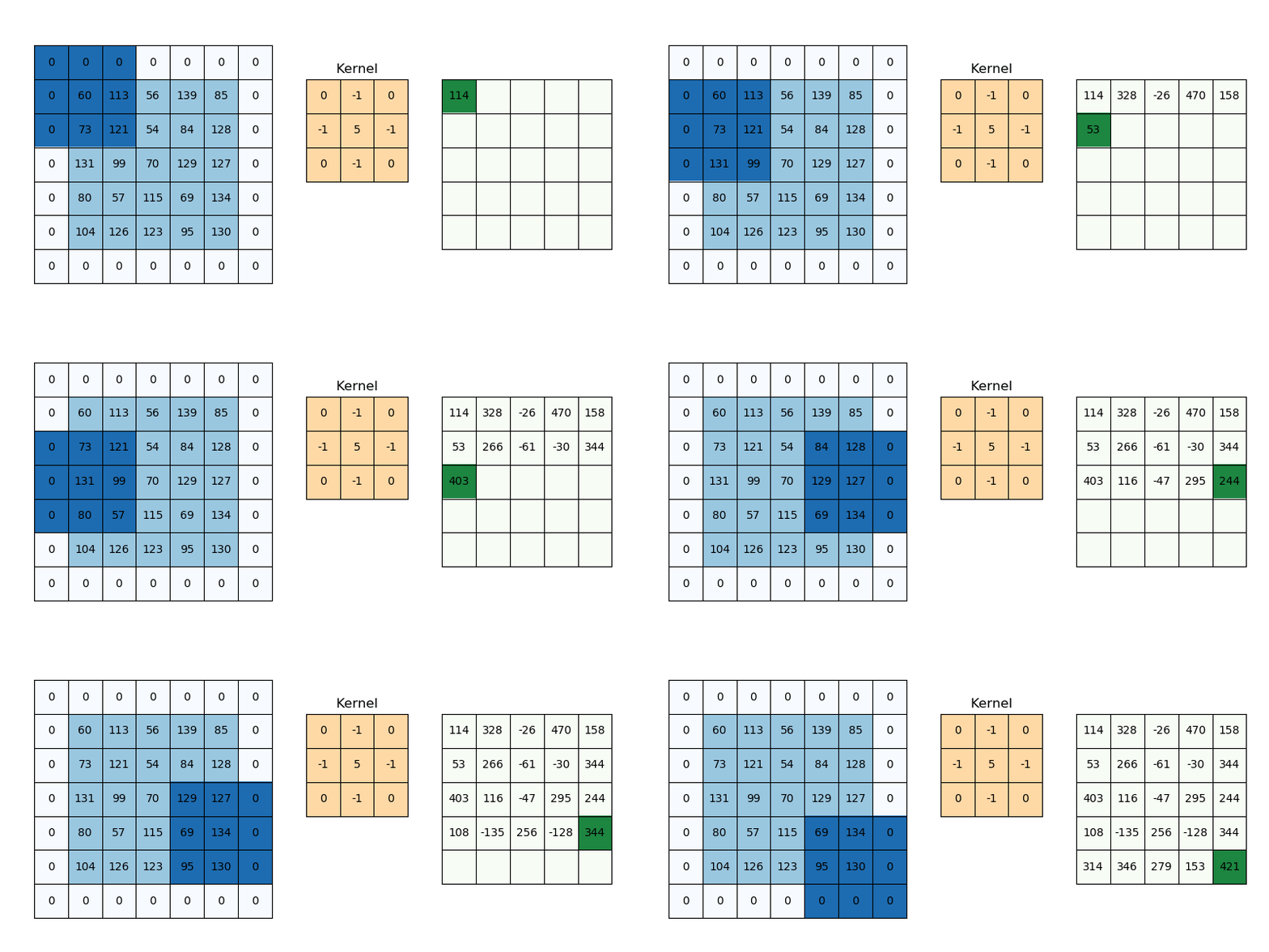
Why Padding is Needed
When applying convolution, the output image shrinks unless we pad it. This is a problem when building deep networks where spatial dimensions shrink after each convolution.
Without Padding:
$$ \text{Output size} = n - f + 1 $$
Where:
- $n$: input size
- $f$: filter size
Example
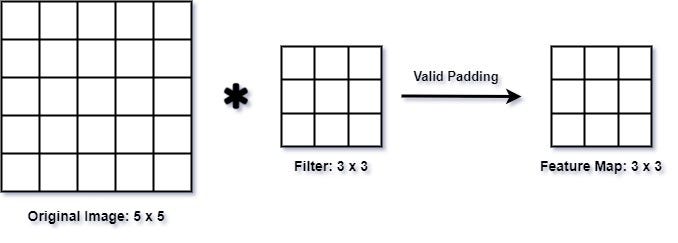
In this image:
- $n$: input size = $5$
- $f$: filter size = $3$
$$ \text{Output size} = n - f + 1 $$
$$ \text{Output size} = 5 - 3 + 1 $$
$$ \text{Output size} = 3 $$
With Padding ($p$):
$$ \text{Output size} = n + 2p - f + 1 $$
Where:
- $n$: input size
- $f$: filter size
- $p$: padding size
Example
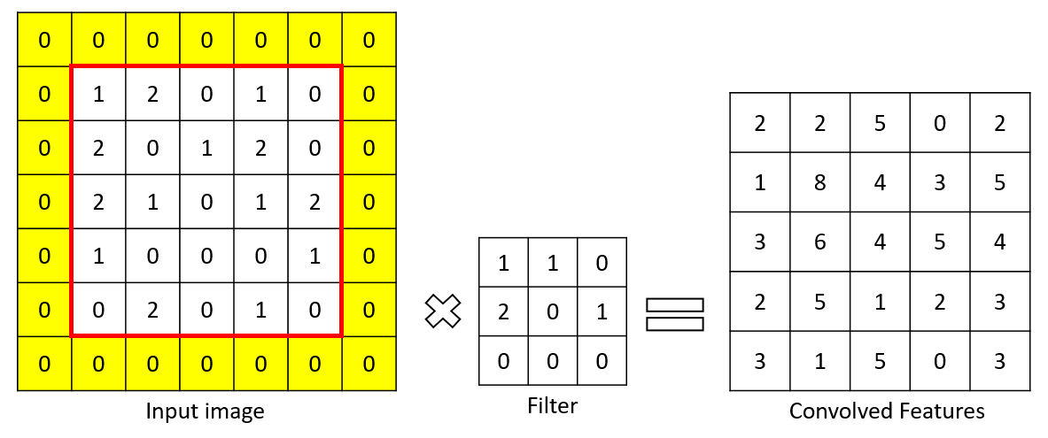
In this image:
- $n$: input size = $6$
- $f$: filter size = $3$
- $p$: padding size = $1$
$$ \text{Output size} = n + 2p - f + 1 $$
$$ \text{Output size} = 6 + (2\cdot 1) - 3 + 1 $$
$$ \text{Output size} = 6 $$
Types of Padding
- Valid Padding (no padding): Output is smaller.
- Same Padding (zero padding): Output size equals input size.
Real-World Analogy
Imagine scanning a photo with a magnifying glass: without padding, you can’t examine the borders. Padding extends the image so that every pixel gets equal attention.
Strided Convolutions
What is Stride?
Stride is the number of pixels the filter moves at each step.
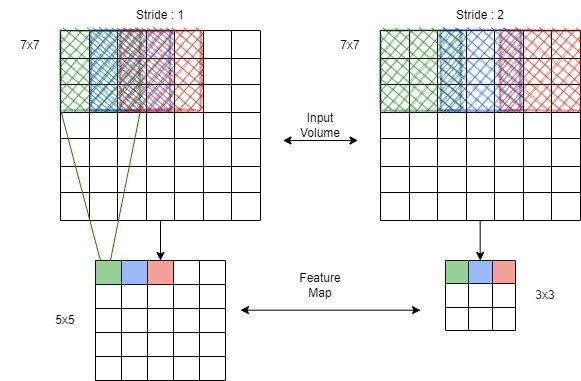
- Stride = 1: Normal convolution (moves 1 pixel at a time)
- Stride = 2: Downsampling (moves 2 pixels at a time)
Output Size Formula
$$ \text{Output size} = \left\lfloor \frac{n + 2p - f}{s} \right\rfloor + 1 $$
Where:
- $n$: input size
- $f$: filter size
- $s$: stride
- $p$: padding
Visual Example
If stride = 2, the filter skips every alternate pixel, effectively reducing the spatial size of the output.
Convolutions Over Volume
From 2D to 3D
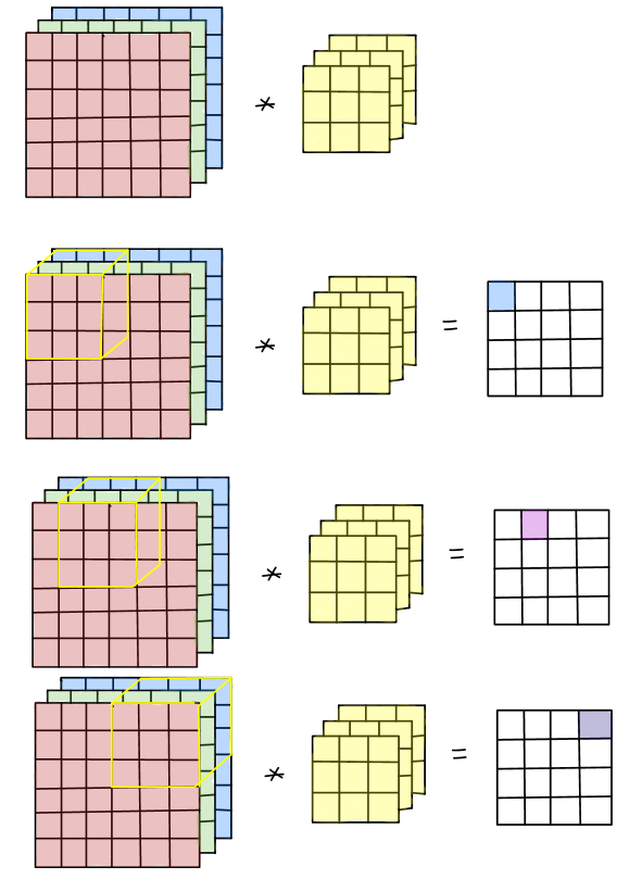
In RGB images, we have 3 channels: Red, Green, and Blue. Thus, a convolutional layer operates over 3D volumes.
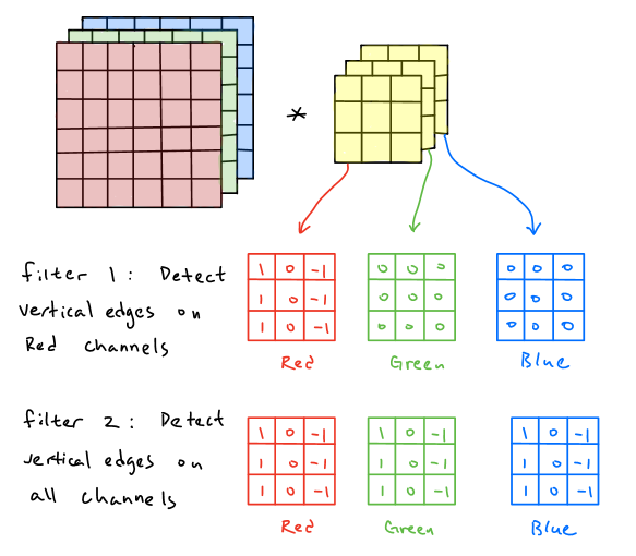
Input Dimensions:
$$ (n_H, n_W, n_C) $$
- $n_H$: Height
- $n_W$: Width
- $n_C$: Channels (e.g., 3 for RGB)
Filter Dimensions:
$$ (f_H, f_W, n_C) $$
- Number of filters: $n_F$
Output Volume:
$$ (n_H’, n_W’, n_F) $$
- Each filter creates a 2D activation map, stacked together to form the output volume.
Practical Example
Let’s say you have a (6, 6, 3) image, and you apply 2 filters of size (3, 3, 3):
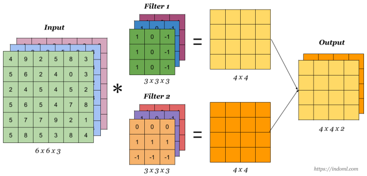
- Output shape: (4, 4, 2) (assuming valid padding, stride=1)
CNN Architecture and Examples
1. One Layer of a Convolutional Network
A Convolutional Neural Network (CNN) is typically composed of three types of layers:
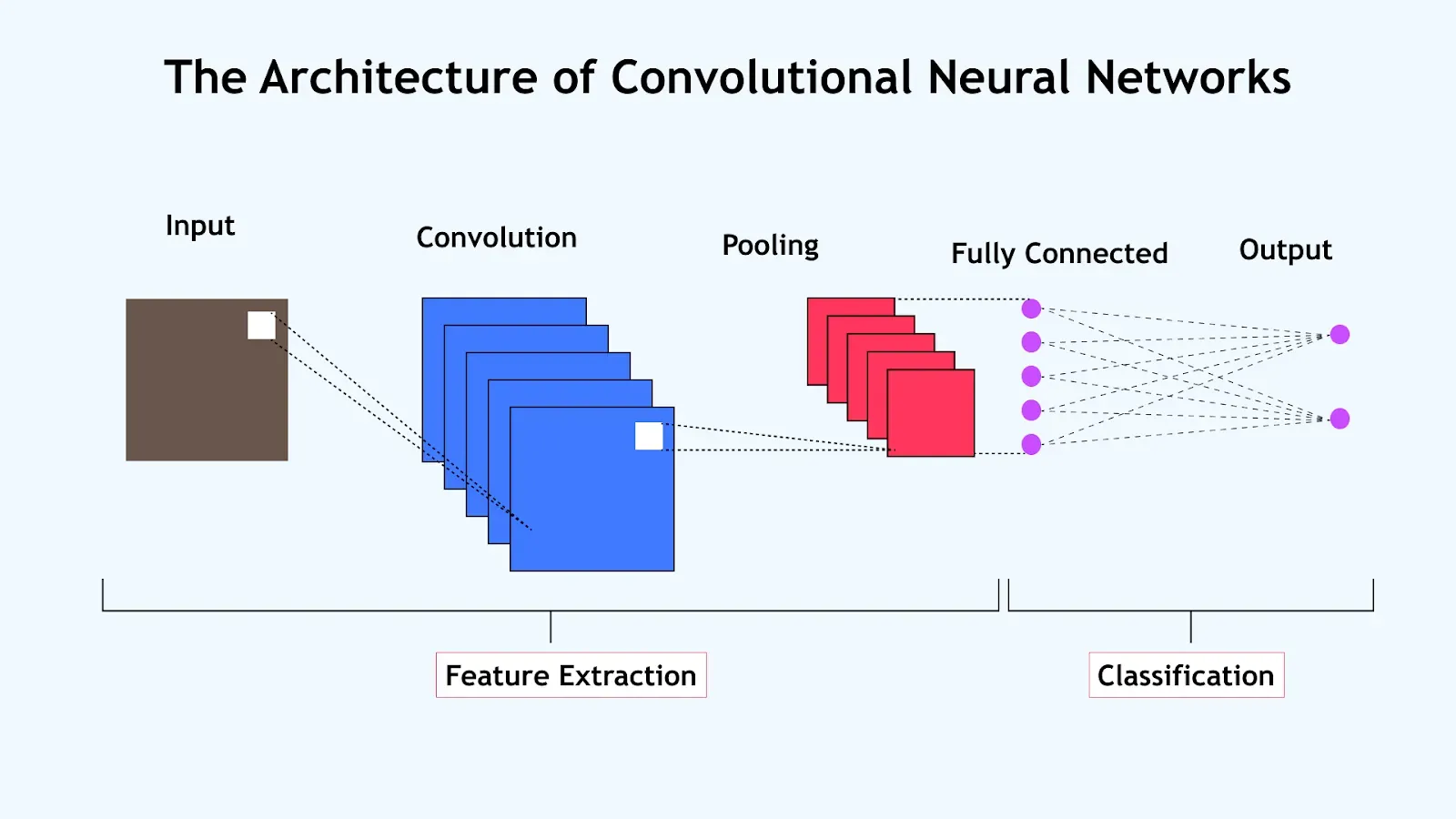
- Convolutional layers: Apply filters to extract spatial features.
- Pooling layers: Downsample feature maps to reduce computation.
- Fully connected layers: Perform final classification or regression.
Each layer transforms the input volume into an output volume through learnable parameters or fixed operations.
Layer Types of CNN
1. Convolutional Layers
Purpose:
To extract spatial features such as edges, textures, and patterns by sliding filters over the input image or feature map.
How it works:
- A filter (or kernel) of size $f \times f$ slides over the input.
- At each location, an element-wise multiplication is performed between the filter and the part of the input it overlaps.
- The results are summed to produce a single number in the output feature map.
Mathematical Operation:
Let the input be $X \in \mathbb{R}^{n_H \times n_W \times n_C}$ and the filter be $W \in \mathbb{R}^{f \times f \times n_C}$.
$$ Z_{i,j} = \sum_{m=0}^{f-1} \sum_{n=0}^{f-1} \sum_{c=0}^{n_C-1} X_{i+m,j+n,c} \cdot W_{m,n,c} + b $$
Example:
Input: $5 \times 5$ grayscale image with $3 \times 3$ filter:
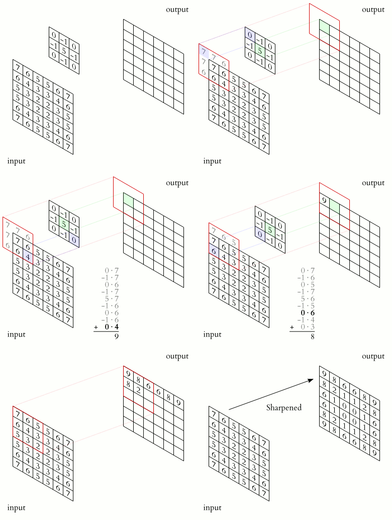
As the filter slides across the input, it detects vertical and horizontal edges by producing high activation in regions with strong center transitions.
2. Pooling Layers
Purpose:
To reduce the spatial dimensions (height and width) of the feature maps, thereby:
- Reducing the number of parameters and computation
- Controlling overfitting
- Making the model invariant to small translations in the input
Types:
Max Pooling:
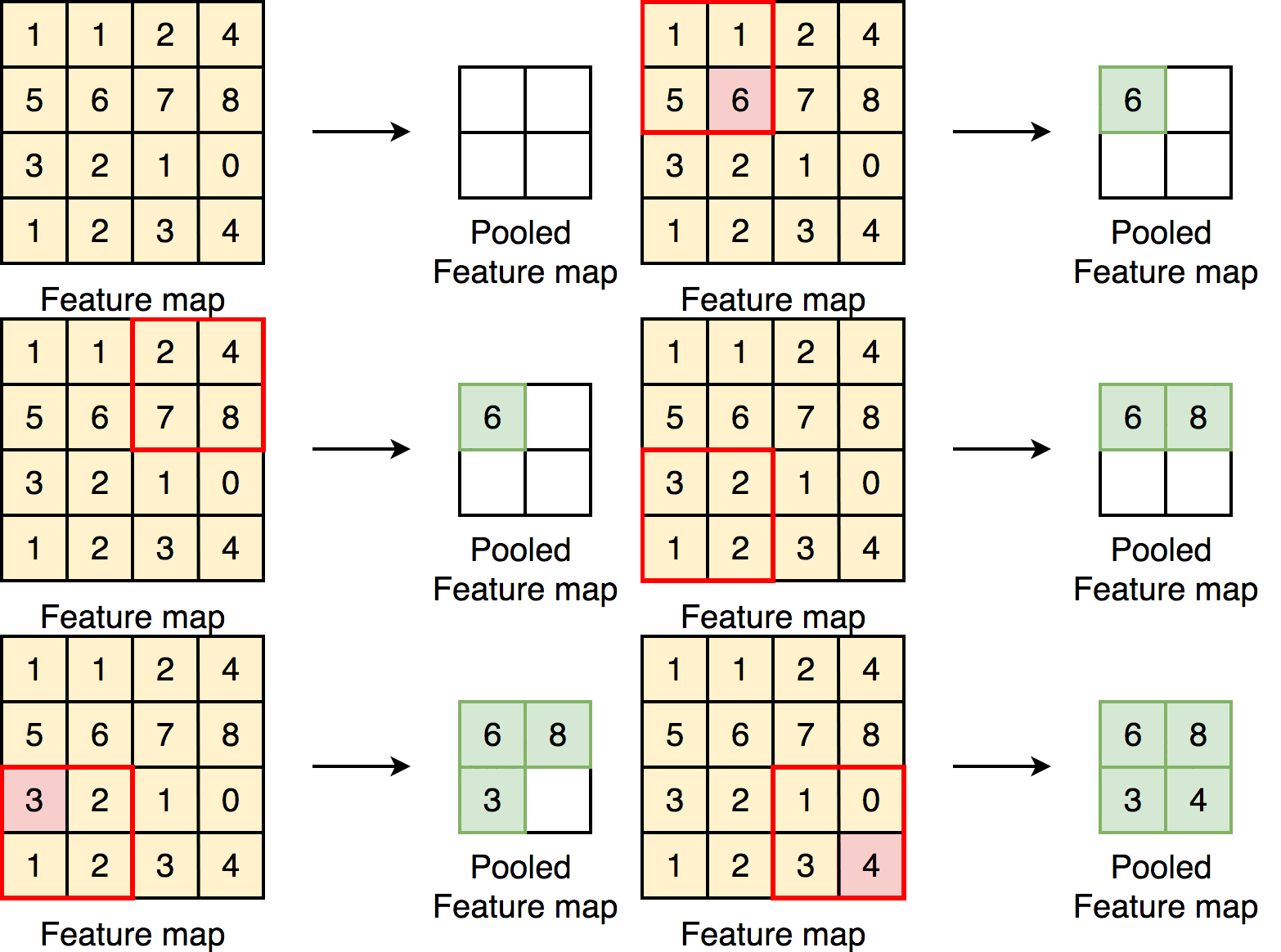
Selects the maximum value in each region.
Average Pooling:
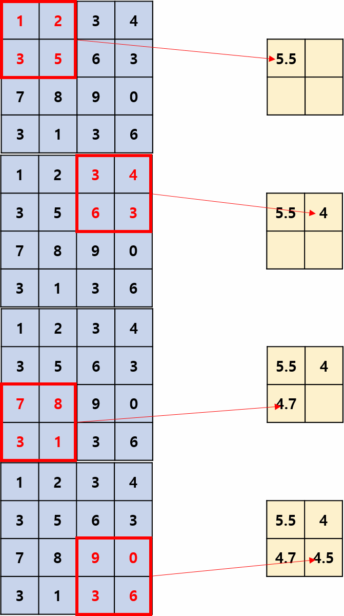
Takes the average of values in each region.
3. Fully Connected Layers
To connect every neuron in one layer to every neuron in the next layer, performing the final classification or regression.
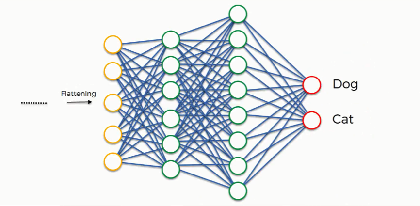
How it works:
- Takes the flattened output from the last convolutional/pooling layer
- Passes it through one or more dense layers
- Final layer often uses softmax for classification
Mathematical Form:
Given the input vector $x \in \mathbb{R}^n$, weights $W \in \mathbb{R}^{m \times n}$, and bias $b \in \mathbb{R}^m$:
$$ z = Wx + b $$
$$ a = g(z) \text{ where } g \text{ is an activation function (e.g., ReLU, Softmax)} $$
Example:
Let’s say we have a feature map output size of $5 \times 5 \times 16 = 400$ from the last pooling layer:
- FC1: 400 → 120 (ReLU)
- FC2: 120 → 84 (ReLU)
- FC3: 84 → 10 (Softmax, for 10-class classification)
These dense layers combine all the high-level features learned in the earlier layers and output a prediction.
Summary Table
| Layer Type | Role | Typical Parameters | Output Shape Transformation |
|---|---|---|---|
| Convolutional | Extract local spatial features | $f$, $s$, $p$, filters | $n_H \times n_W \times n_C \rightarrow n_{H’} \times n_{W’} \times n_{C’}$ |
| Pooling | Downsample feature maps | $f$, $s$ | $n_H \times n_W \times n_C \rightarrow n_{H’} \times n_{W’} \times n_C$ |
| Fully Connected | Final classification/regression | neurons per layer | $n \rightarrow m$ (vector size) |
These layers together form the foundation of Convolutional Neural Networks, enabling them to learn hierarchical representations from raw pixels to abstract concepts.
Notation and Terminology
- $ n_H, n_W $: height and width of the input volume
- $ n_C $: number of channels (depth)
- $ f $: filter size
- $ s $: stride
- $ p $: padding
- $ W^{[l]} $, $ b^{[l]} $: weights and biases at layer $ l $
Parameters and Learnable Components
- Weights ($ W $): Represent filters; shared spatially across the input.
- Biases ($ b $): One per filter.
- Activation ($ A $): Output of ReLU or other non-linear function.
Each neuron in a layer is connected only to a small region of the previous layer, leading to sparse interactions and parameter sharing.
3. CNN Example (Comprehensive Network)
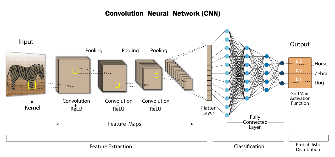
Why Convolutions?
Convolutional layers are the cornerstone of modern deep learning models in computer vision, replacing traditional fully connected layers in image tasks. This section explores why convolutions are used instead of dense layers, and what advantages they bring.
1. The Limitations of Fully Connected Layers for Images
a. Parameter Explosion
A fully connected (dense) layer connecting every pixel of an image to every neuron in the next layer requires a huge number of parameters.
Example:
- Input image size: $ 64 \times 64 \times 3 = 12,288 $
- Fully connected layer with 1000 neurons: $ \text{Parameters} = 12,288 \times 1000 = 12,288,000 $
This leads to high memory usage, overfitting risk, and long training times.
b. Ignores Spatial Structure
Dense layers treat input features independently and do not take advantage of the spatial locality of image data.
- A cat’s ear in the top-left and bottom-right corners are treated as unrelated by dense layers.
2. Benefits of Convolutional Layers
a. Sparse Interactions
Each output neuron is connected only to a small region of the input (called the receptive field).
- Fewer parameters
- Faster computations
Example:
- Using $ f = 5 $ instead of connecting all 12,288 pixels
b. Parameter Sharing
Same filter (weights) is applied across the entire image:
$$ Z[i, j] = \sum_{m=0}^{f-1} \sum_{n=0}^{f-1} W[m, n] \cdot X[i+m, j+n] + b $$
This results in drastic reduction in number of parameters and allows feature detection to be translation invariant.
c. Translation Equivariance
- If an object moves in the image, its feature map also moves.
- The model learns position-independent features — important for generalization.
Classic Networks: LeNet-5, AlexNet, VGG
- Why Look at Classic Networks?
- LeNet-5 (1998, Yann LeCun)
- AlexNet (2012, Alex Krizhevsky, Ilya Sutskever, Geoffrey Hinton)
- VGG Networks (2014, Visual Geometry Group, Oxford)
- Summary Table
- Final Thoughts
In the early stages of deep learning and computer vision, several foundational convolutional neural network (CNN) architectures shaped the field and enabled significant breakthroughs in image recognition. In this document, we explore three of the most historically significant and technically influential networks: LeNet-5, AlexNet, and VGG.
These architectures demonstrate the progression of CNN design from shallow, simple models to deeper, more powerful systems capable of scaling to large datasets like ImageNet.
Why Look at Classic Networks?
Understanding classic CNN architectures is essential for the following reasons:
- They introduce fundamental building blocks (e.g., convolutional layers, pooling layers, ReLU activation).
- They highlight challenges faced at different stages of deep learning evolution (e.g., overfitting, vanishing gradients).
- They provide insights into the design philosophy of modern deep architectures.
LeNet-5 (1998, Yann LeCun)
Overview
LeNet-5 was one of the earliest CNN models designed to recognize handwritten digits (e.g., MNIST dataset). It demonstrated the power of learned convolutional filters combined with a small number of parameters.
Architecture
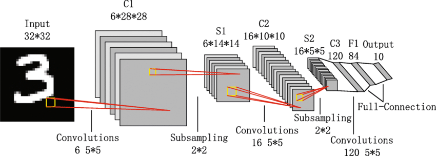
- Input: 32x32 grayscale image
- C1: Convolutional layer with 6 filters of size 5x5 → output: 28x28x6
- S2: Subsampling (average pooling) layer → output: 14x14x6
- C3: Convolutional layer with 16 filters → output: 10x10x16
- S4: Subsampling layer → output: 5x5x16
- C5: Fully connected convolutional layer → output: 120
- F6: Fully connected layer → output: 84
- Output: 10-class softmax layer
Parameters
LeNet uses shared weights, reducing the number of parameters compared to fully connected networks.
Insights
- Introduced the idea of local receptive fields, weight sharing, and subsampling.
- Excellent for small datasets but struggles with large-scale data due to its shallow depth.
AlexNet (2012, Alex Krizhevsky, Ilya Sutskever, Geoffrey Hinton)
Breakthrough
AlexNet marked the first major success of deep learning in the ImageNet Large Scale Visual Recognition Challenge (ILSVRC 2012), achieving top-5 error of 15.3%, compared to 26% for the runner-up.
Architecture
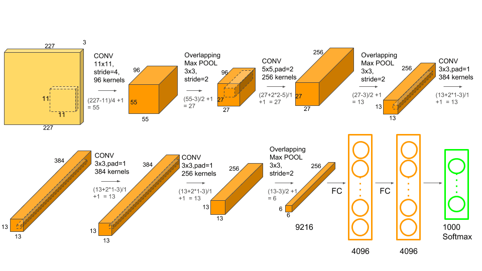
- Input: 224x224x3 RGB image
- Conv1: 96 filters of 11x11, stride 4 → 55x55x96
- MaxPool1: 3x3, stride 2 → 27x27x96
- Conv2: 256 filters of 5x5 → 27x27x256
- MaxPool2: 3x3 → 13x13x256
- Conv3: 384 filters of 3x3 → 13x13x384
- Conv4: 384 filters of 3x3 → 13x13x384
- Conv5: 256 filters of 3x3 → 13x13x256
- MaxPool3: 3x3 → 6x6x256
- FC6: Fully connected layer with 4096 neurons
- FC7: Fully connected layer with 4096 neurons
- FC8: 1000-way softmax layer
Key Innovations
- Used ReLU (Rectified Linear Unit) instead of sigmoid or tanh → faster training
- Introduced dropout for regularization
- Trained on two GPUs in parallel
Insights
- Showed the world that deep networks could outperform traditional machine learning models if trained with large datasets and GPUs.
VGG Networks (2014, Visual Geometry Group, Oxford)
VGG emphasized simplicity and depth: using small 3x3 filters and stacking them deeply to capture complex patterns.
Architecture (VGG-16)
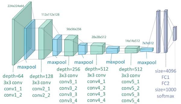
- Input: 224x224x3 RGB image
- Stack of 13 convolutional layers using 3x3 filters
- 5 max-pooling layers to reduce spatial dimensions
- 3 fully connected layers, with the last one as a softmax for classification
Example:
- Conv3-64 → Conv3-64 → MaxPool
- Conv3-128 → Conv3-128 → MaxPool
- Conv3-256 → Conv3-256 → Conv3-256 → MaxPool
- Conv3-512 → Conv3-512 → Conv3-512 → MaxPool
- Conv3-512 → Conv3-512 → Conv3-512 → MaxPool
- FC-4096 → FC-4096 → Softmax(1000)
Characteristics
- Consistent use of 3x3 filters simplifies the design and enables deeper networks
- Requires significant memory and computation (hundreds of millions of parameters)
Insights
- Demonstrated that depth is a key factor in improving CNN performance
- The architecture became a benchmark and inspired many follow-up models
Summary Table
| Model | Year | Input Size | Depth | Unique Aspects |
|---|---|---|---|---|
| LeNet-5 | 1998 | 32x32 | 7 | Local receptive fields, subsampling |
| AlexNet | 2012 | 224x224x3 | 8 | ReLU, dropout, GPU parallelism |
| VGG-16 | 2014 | 224x224x3 | 16 | Simplicity, 3x3 filters, depth |
Final Thoughts
These classic CNN architectures form the backbone of modern computer vision systems. Each contributed key architectural innovations that addressed specific challenges in training deep networks.
Understanding them allows us to appreciate the evolution of deep learning and to better design models suited for today’s massive data and compute resources.
Modern CNN Architectures: ResNet, Inception, MobileNet, EfficientNet
ResNet: Deep Residual Networks
As neural networks became deeper, researchers observed a counterintuitive phenomenon: deeper networks often performed worse during training and testing compared to shallower ones. This degradation was not due to overfitting but rather an optimization issue.
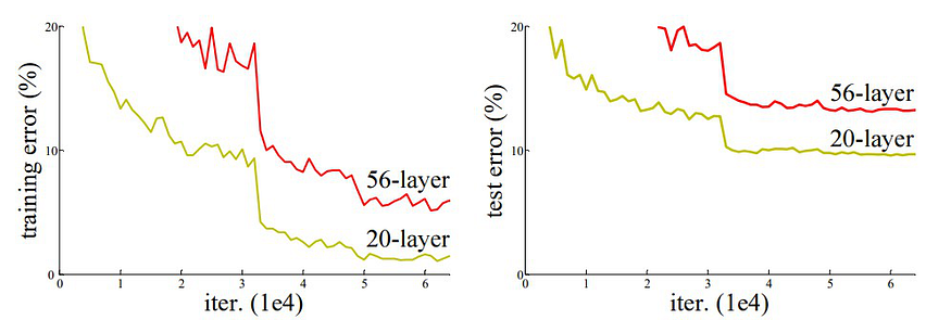
This problem is called the degradation problem. It shows that simply stacking more layers doesn’t guarantee better accuracy — instead, it often leads to higher training error. This contradicts our expectations, since deeper models should be able to represent more complex functions.
To address this, ResNet introduced the concept of residual learning.
Residual Learning: Core Idea
Instead of learning a direct mapping $ H(x) $, ResNet proposes to learn the residual function:
$$ F(x) = H(x) - x \Rightarrow H(x) = F(x) + x $$
This reformulation allows the network to focus on learning the difference between the input and output, which is often easier to optimize.
The output of a residual block is:
$$ \text{Output} = F(x, {W_i}) + x $$
where $ F(x, {W_i}) $ is the output from a few stacked layers (e.g., 2 Conv-BN-ReLU layers) and $ x $ is the original input. This addition is known as a skip connection or shortcut connection.
Here’s the basic structure of a Residual Block:
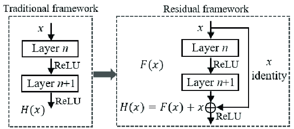
- If the input and output dimensions differ, a 1x1 convolution is used to match dimensions before addition.
- This structure allows gradients to flow more easily during backpropagation, mitigating the vanishing gradient problem.
Identity Shortcut Connection
This is the key innovation. By allowing the input to bypass intermediate layers, the model can preserve useful features, learn identity mappings when needed, and avoid overfitting.
Shortcut types:
- Identity shortcut: When input and output dimensions match
- Projection shortcut: 1x1 convolution used to match shapes
Why ResNets Work?
- Improved Gradient Flow: Easier to train deep networks due to unblocked gradient paths
- Easier Optimization: Residual mapping simplifies the learning process
- Deeper Networks: Can train very deep networks (e.g., ResNet-152) without degradation
- Better Generalization: Performs well across image classification, detection, segmentation
Forward and Backward Propagation
In a residual block, during forward propagation, the shortcut allows direct data flow from earlier layers. In backward propagation, the gradient can pass through both the residual path and shortcut connection, reducing gradient vanishing.
Let’s say the loss gradient is $ \partial L/\partial y $. Then:
$$ \frac{\partial L}{\partial x} = \frac{\partial L}{\partial y} \cdot (\frac{\partial F}{\partial x} + I) $$
Here, $ I $ is the identity matrix, ensuring that gradient doesn’t vanish even if $ \partial F/\partial x $ becomes small.
Real-World Analogy
Imagine you’re assembling a piece of furniture using instructions. Instead of reading and understanding every step from scratch (direct mapping), you compare each step with what you’ve already done (residual comparison). It’s easier to notice what’s missing and fix it.
Variants of ResNet
- ResNet-18, 34, 50, 101, 152: Increasing depth
- ResNeXt: Groups of convolutions
- Pre-activation ResNet: Moves BN and ReLU before convolutions
Inception and 1x1 Convolutions
Networks in Networks and 1x1 Convolutions
In 2014, the “Network in Network” architecture introduced the idea of using 1x1 convolutions — a surprisingly powerful and efficient technique in modern CNNs.
What is a 1x1 Convolution?
- A 1x1 convolution applies a filter of size $1×1$ across all input channels.
- Though the spatial dimension ($1x1$) seems trivial, it processes channel-wise information and mixes features across depth.
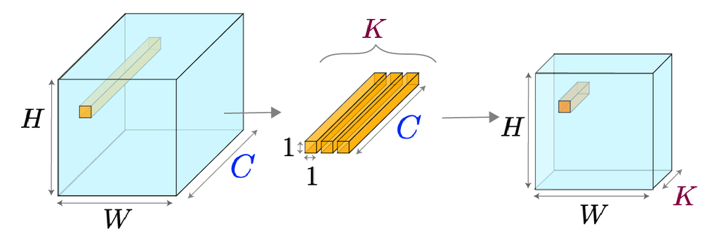
Let’s assume an input of shape $ H \times W \times C_{in}$. Applying $ N $ 1x1 filters produces an output of shape $ H \times W \times N $.
Why is it useful?
- Dimensionality Reduction: You can reduce the number of channels before applying computationally expensive filters (e.g., 3x3, 5x5), reducing the model size and speed requirements.
- Increase Non-Linearity: When combined with non-linear activations (like ReLU), it increases the representational power of the network.
- Lightweight Computation: Compared to a standard 3x3 convolution with the same input/output dimensions, the FLOPs (floating point operations) required are significantly lower.
Intuition:
Think of 1x1 convolution as a way to relearn combinations of channels at each spatial location. It’s like assigning weights to each feature and mixing them in a smart way — like forming new meanings from known “ingredients.”
Inception Network
CNNs originally used sequential layers — stacking 3x3 or 5x5 filters one after another. But why settle for a single filter size?
Some patterns might be better captured with:
- 1x1 (fine details)
- 3x3 (mid-level features)
- 5x5 (larger context)
Key Insight:
Why not apply all of them in parallel, and let the network decide which one is best?
That’s the core idea behind the Inception Module.
Problem:
Applying multiple large filters in parallel increases computation exponentially.
GoogLeNet and Inception Blocks
The GoogLeNet (Inception-v1) architecture introduced the Inception module to allow multi-scale feature extraction while keeping the computation affordable.
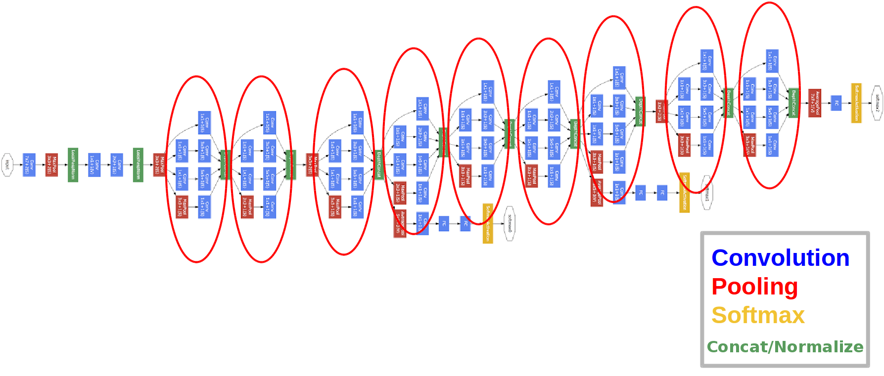
Structure of an Inception Block:
Each Inception block has multiple branches:
- 1x1 convolution
- 1x1 → 3x3 convolution
- 1x1 → 5x5 convolution
- 3x3 max pooling → 1x1 convolution
Notice how each expensive convolution is preceded by a 1x1 convolution for dimensionality reduction.
Advantages:
- Parameter Efficiency: Fewer parameters than naïvely stacking all filters.
- Rich Feature Learning: Learns features at multiple receptive fields simultaneously.
- Parallelism: More effective than deeper or wider models with uniform layers.
Example:
Assume an input of size $ 28 \times 28 \times 192 $. After passing through an Inception module, we may get something like:
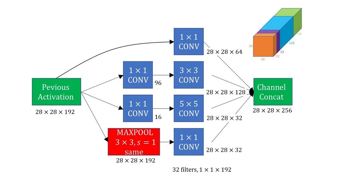
- 1x1 branch → 64 channels
- 3x3 branch → 128 channels
- 5x5 branch → 32 channels
- Pooling branch → 32 channels
- Total output depth: 256
Improvements Over Time
GoogLeNet inspired many improved versions:
- Inception v2/v3: Factorization of convolutions (e.g., 5x5 → two 3x3 layers)
- Inception v4: Combined ideas from ResNet and Inception (e.g., Inception-ResNet)
- Use of BatchNorm and Auxiliary Classifiers
These tricks improved accuracy without dramatically increasing parameters.
The Inception architecture was a major leap forward in CNN design:
- It introduced the concept of multi-path architectures
- Emphasized computational efficiency
- Leveraged 1x1 convolutions to control model complexity
This paved the way for even more efficient models like MobileNet and EfficientNet.
MobileNet and EfficientNet
MobileNet
As deep learning models became larger and deeper, they demanded more memory and computation — not ideal for mobile or embedded devices. MobileNet, introduced by Google in 2017, addressed this challenge by proposing a highly efficient architecture using depthwise separable convolutions.
Standard Convolution vs. Depthwise Separable Convolution
Let’s recall the standard convolution:
Given an input of size $ H \times W \times D_{in} $, applying $ N $ filters of size $ K \times K \times D_{in} $ produces an output of size $ H’ \times W’ \times N $.
- Computation Cost: $$ K \cdot K \cdot D_{in} \cdot N \cdot H’ \cdot W’ $$
MobileNet factorizes this into two steps:
-
Depthwise Convolution:
Apply one filter per input channel — no cross-channel combination.
Cost:$$ K \cdot K \cdot D_{in} \cdot H’ \cdot W’ $$
-
Pointwise Convolution (1x1):
Mix the depthwise output with $ N $ 1x1 filters.
Cost: $$ D_{in} \cdot N \cdot H’ \cdot W’ $$
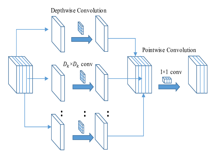
✅ Total Cost:
$$ K^2 \cdot D_{in} \cdot H’ \cdot W’ + D_{in} \cdot N \cdot H’ \cdot W’ $$
which is ~9x less than standard convolution when $ K = 3 $.
MobileNet Architecture (V1 Highlights)
MobileNetV1 is built by stacking depthwise separable convolutions instead of regular ones. It also introduces:
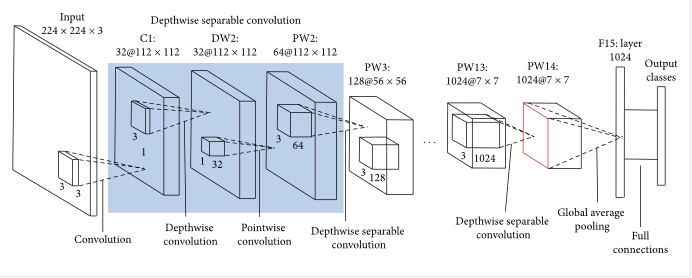
- Width Multiplier (α): Shrinks the number of channels (e.g., α=0.75 reduces model size).
- Resolution Multiplier (ρ): Reduces input image size to further save computation.
Together, these enable a trade-off between accuracy and resource usage.
MobileNet is often used as a backbone in real-time applications (e.g., object detection on smartphones, AR apps).
EfficientNet
Introduced in 2019 by Google AI, EfficientNet pushes the boundary of model performance by scaling neural networks systematically.
The Problem: How to Scale a CNN?
You can make a CNN more powerful by:
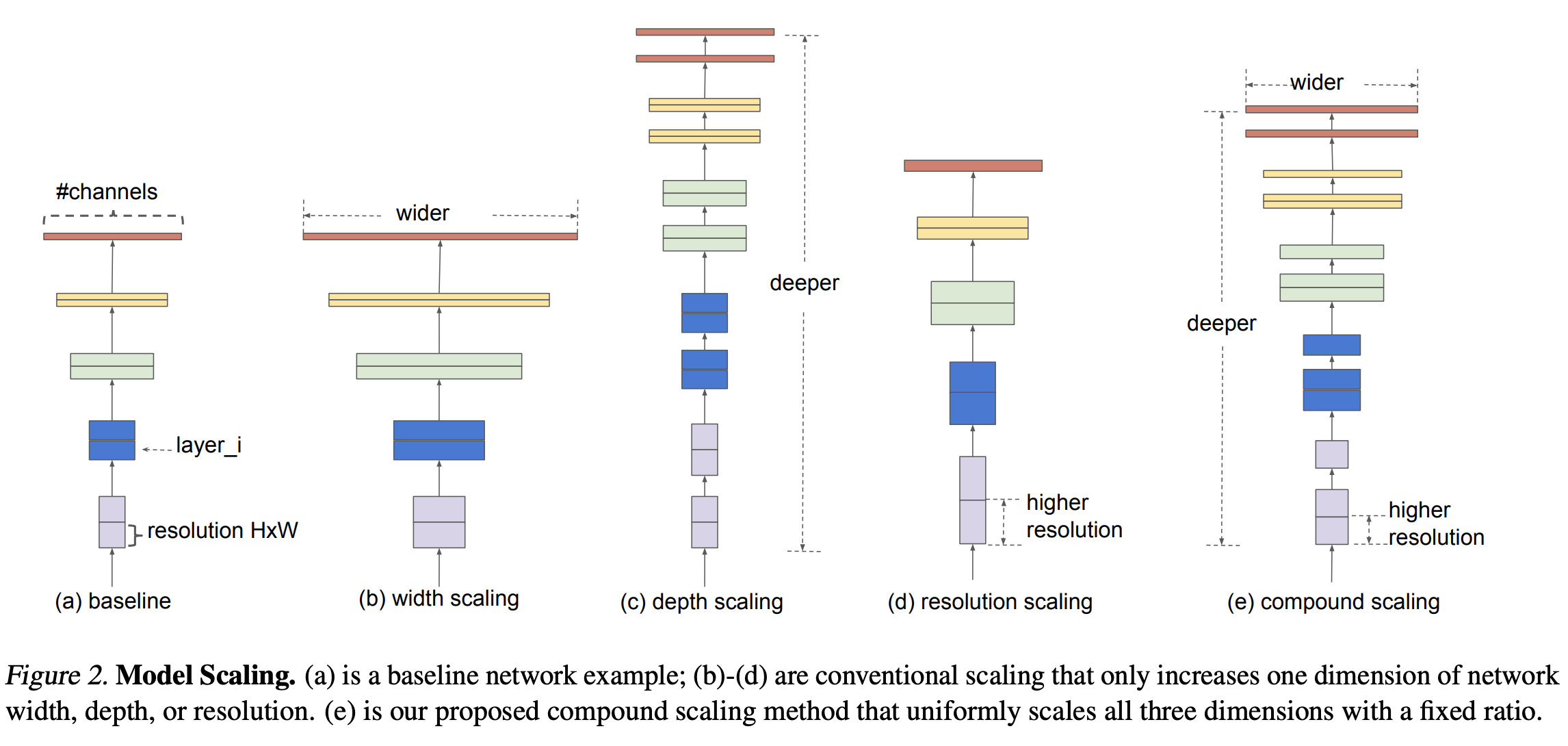
- Increasing depth (more layers)
- Increasing width (more channels)
- Increasing resolution (larger input images)
But how much of each?
Compound Scaling: Efficient Strategy
Instead of arbitrarily scaling one dimension, EfficientNet introduces a compound coefficient (ϕ) that balances all three:
$$ \begin{aligned} \text{depth:} &\quad d = \alpha^\phi \ \text{width:} &\quad w = \beta^\phi \ \text{resolution:} &\quad r = \gamma^\phi \ \text{subject to:} &\quad \alpha \cdot \beta^2 \cdot \gamma^2 \approx 2 \end{aligned} $$
- ϕ controls the available resources (e.g., more computation).
- α, β, γ are constants determined via grid search.
Performance
EfficientNet models (B0 to B7) are built on the same base architecture (EfficientNet-B0), with progressively larger values of ϕ.
- EfficientNet-B0: baseline
- EfficientNet-B1 to B7: scaled versions with increasing capacity
✅ Result:
EfficientNet achieves better accuracy with fewer parameters compared to deeper networks like ResNet-152 or Inception-v4.
| Architecture | Key Idea | Efficiency Trick |
|---|---|---|
| MobileNet | Lightweight model for mobile | Depthwise separable convolutions |
| EfficientNet | Scalable and accurate model | Compound scaling across depth, width, resolution |
Both architectures represent the evolution of CNN design towards compact, fast, and powerful models — a necessary shift for real-world AI deployment.
Object Localization and Detection
- Object Localization
- Landmark Detection
- Object Detection
- Sliding Window Approach and Its Convolutional Implementation
Object Localization
Object localization is the task of identifying the presence of an object in an image and determining its position using a bounding box.
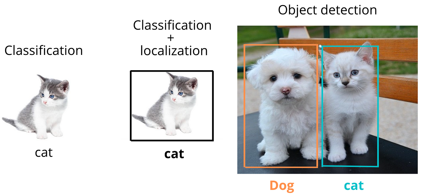
It’s one step more complex than image classification, which only tells what is in the image, not where it is.
Given an image, object localization aims to:
- Classify the object (e.g., cat, dog, car).
- Return the bounding box coordinates around the object: $$ (x_{\text{min}}, y_{\text{min}}, x_{\text{max}}, y_{\text{max}}) \quad \text{or} \quad (x, y, w, h) $$
Where:
- $ (x, y) $: center of the bounding box
- $ w, h $: width and height of the box
Output Vector
If you’re using a neural network for localization, the output vector might be:
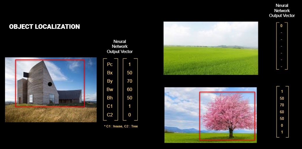
$$ \text{Output} = [p_c, x, y, w, h, c_1, c_2, …, c_n] $$
Where:
- $ p_c $: Probability that an object exists in the image
- $ x, y, w, h $: Bounding box
- $ c_i $: Class probabilities (e.g., cat = 0.8, dog = 0.2)
If the object whose class is defined cannot be detected on the image, $p_c$ will be $0$. In the case where $p_c$ is $0$, the bounding box values ($x ,y, w, h$) and class values are insignificant in the vector. This means that they are not included when calculating the Loss function.
Loss Function
A multi-part loss is generally used for localization:
- Localization loss (coordinate regression): Measures error in predicted box location
- Confidence loss (objectness): Measures error in object existence
- Classification loss: Measures class prediction error
Example (simplified version as in YOLO):
$$ \mathcal{L} = \lambda_{\text{coord}} \cdot \sum_{i} \mathbb{1}_{i}^{\text{obj}} \left[(x_i - \hat{x}_i)^2 + (y_i - \hat{y}_i)^2 + (w_i - \hat{w}_i)^2 + (h_i - \hat{h}_i)^2\right] + \text{classification loss} $$
Landmark Detection
Landmark detection (also called keypoint detection) involves detecting specific key locations on an object. Unlike bounding boxes, keypoints give finer-grained localization.
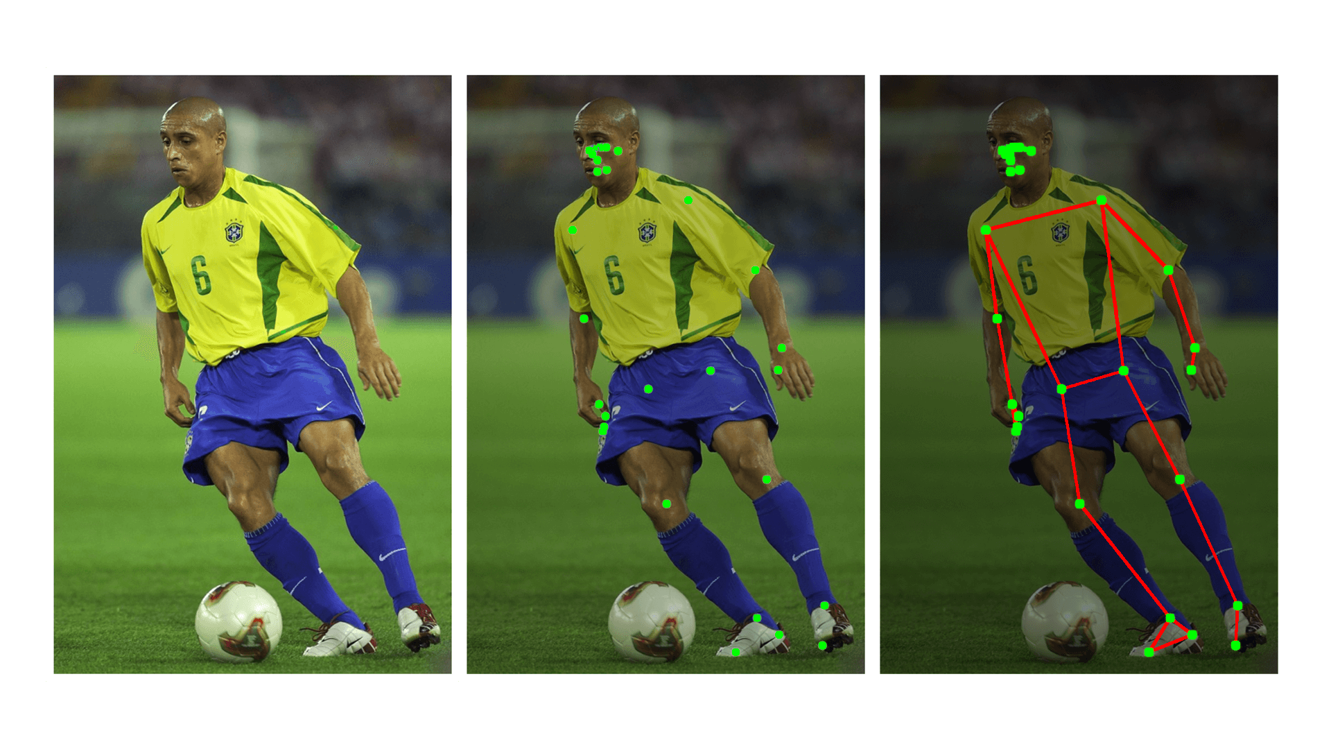
Example
- Face recognition: Eyes, nose tip, mouth corners
- Hand detection: Fingertips and joints
- Medical imaging: Identifying organ boundaries
Output Representation
If we detect $ K $ landmarks:
$$ \text{Output} = [x_1, y_1, x_2, y_2, …, x_K, y_K] $$
Each pair represents the $(x, y)$ coordinate of a keypoint like knee point or ear point.
Loss Function
The typical loss for landmark detection:
$$ \mathcal{L}{\text{keypoints}} = \sum{k=1}^{K} \left[(x_k - \hat{x}_k)^2 + (y_k - \hat{y}_k)^2\right] $$
Object Detection
Object detection combines classification and localization — but now for multiple objects in the same image.
Example
In a single street photo:
- Detect a car (class = car, bounding box)
- Detect a pedestrian (class = human, bounding box)
- Detect a stop sign (class = sign, bounding box)
Compared to Localization
| Task | Output |
|---|---|
| Classification | Class label |
| Localization | Class + bounding box |
| Detection | Multiple classes + boxes |
Model Output Structure
We divide the image into an $ S \times S $ grid. For each grid cell, predict:
- $ B $ bounding boxes
- Confidence score
- Class probabilities
$$ \text{Output Tensor} = S \times S \times (B \cdot 5 + C) $$
Where:
- Each box includes $[p_c, x, y, w, h]$. $5$ means this vector.
- $ C $: number of classes
Sliding Window Approach and Its Convolutional Implementation
The sliding window technique is a classic method in computer vision used for object detection. The core idea is to take a fixed-size rectangular window and slide it across the input image, systematically checking each region to see whether it contains the object of interest.
At each window position, the cropped image region is passed to a classifier (e.g., SVM, logistic regression, or a small CNN) to determine whether it contains an object. This window “slides” over the image both horizontally and vertically, often with some stride value, producing many cropped regions.
It converts a classification model into a localization tool by brute-force scanning over all possible positions.
Limitations of Naive Sliding Windows
Although conceptually simple, the naive sliding window method has serious drawbacks:
1. High Computational Cost
- For an image of size $ W \times H $, using a window of size $ w \times h $ with stride $ s $, the number of windows is: $$ \left(\frac{W - w}{s} + 1\right) \cdot \left(\frac{H - h}{s} + 1\right) $$ This can result in thousands of regions even for medium-sized images.
- Each window requires a separate forward pass through the classifier network, resulting in massive redundancy since overlapping windows share most of their pixels.
2. Difficulty in Handling Multiple Scales
- Objects in an image can appear at different scales and aspect ratios.
- To address this, either the image must be resized many times or the window size must vary — both of which further increase computation.
3. Fixed Window Shape
- Sliding windows generally use a fixed aspect ratio and size, which makes them less effective for detecting objects with irregular shapes.
Convolutional Implementation of Sliding Windows
To overcome these inefficiencies, modern approaches use the convolutional structure of neural networks to implement the sliding window more efficiently.
Key Insight: Convolutions as Shared Computation
Instead of running the classifier separately on each window, we can:
- Pass the entire image through the convolutional layers of a CNN once
- These layers produce a feature map where each spatial position encodes information about a local receptive field (i.e., a subregion of the image)
- This naturally simulates a sliding window operation
Then, we apply 1x1 convolutions or fully connected layers converted into convolutions over the feature map to produce dense predictions for object presence.
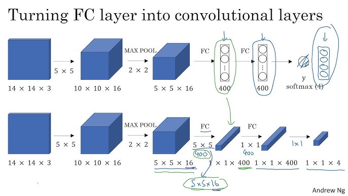
Fully Connected Layer to Convolution
A fully connected layer expecting a flattened $ N \times N \times D $ input can be rewritten as a 1x1 convolution over a $ N \times N \times D $ feature map:
- Each position in the resulting output map corresponds to a specific receptive field on the original image
- This effectively implements classification over many regions at once, reusing shared computation
Use in Modern Architectures
Understanding the YOLO (You Only Look Once) Architecture
YOLO (You Only Look Once) is a real-time object detection system that reframes object detection as a single regression problem, rather than a classification or region proposal problem. Instead of scanning the image multiple times or generating multiple proposals, YOLO sees the entire image only once and directly outputs bounding boxes and class probabilities in a single evaluation.
This end-to-end architecture enables extremely fast inference and is designed for real-time applications such as self-driving cars, robotics, surveillance, and augmented reality.
How Does YOLO Work?
At a high level, YOLO divides the input image into a fixed-size grid and makes predictions for each grid cell. Let’s go through each part of the architecture:
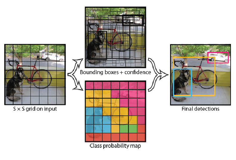
1. Image Grid Division
- The input image is divided into an $ S \times S $ grid (e.g., $ 7 \times 7 $).
- Each grid cell is responsible for detecting objects whose center falls inside the cell.
2. Bounding Box Predictions
Each grid cell predicts:
- $ B $ bounding boxes (typically $ B = 2 $)
- For each box:
- $ x, y $: coordinates of the box center (relative to the grid cell)
- $ w, h $: width and height of the box (relative to the whole image)
- $ p_c $: confidence score = $ P(\text{object}) \times \text{IoU} {\text{pred,truth}} $
3. Class Probabilities
-
Each grid cell also predicts $ C $ conditional class probabilities:
$$ P(\text{class}_i \mid \text{object}) \quad \text{for } i = 1, \dots, C $$
-
These probabilities are class probabilities conditioned on the presence of an object in the cell.
4. Final Predictions
- The total output per grid cell is: $$ B \times [p_c, x, y, w, h] + C $$ For example, with $ S = 7 $, $ B = 2 $, $ C = 20 $, the total prediction tensor size is: $$ 7 \times 7 \times (2 \times 5 + 20) = 7 \times 7 \times 30 $$
Why Is It Called “You Only Look Once”?
Traditional detection pipelines involve:
- Generating region proposals (like in R-CNN)
- Running a CNN on each region
- Performing classification and box regression separately
YOLO unifies this pipeline into a single CNN pass, hence the name “You Only Look Once”. The model sees the full image context and outputs all bounding boxes and class scores in one go.
SSD (Single Shot MultiBox Detector)
- Detects objects at multiple scales using feature maps from different layers
- Uses convolutional layers to predict class and box offsets at every location in the feature map
Summary
| Approach | Characteristics |
|---|---|
| Naive Sliding Window | Slow, inefficient, redundant computation |
| Convolutional Sliding | Efficient, shared computation, suitable for real-time detection |
By understanding this transition from brute-force scanning to convolutional prediction, we appreciate how convolutional networks not only recognize what is in an image but also where, enabling scalable object detection.
Evaluation and Optimization: IoU, Non-max Suppression, Anchor Boxes
Intersection over Union (IoU)
Intersection over Union (IoU) is a metric used to evaluate the accuracy of an object detector on a particular dataset. It measures the overlap between two bounding boxes:
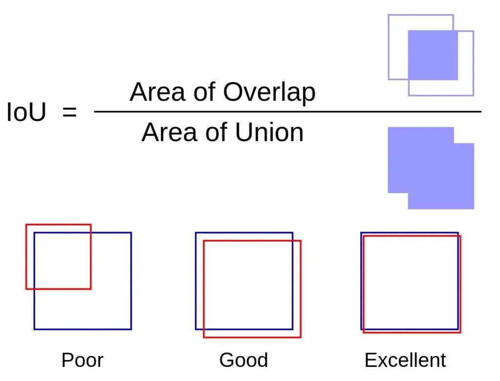
- The predicted bounding box
- The ground-truth bounding box
Mathematical Definition
If $B_p$ is the predicted bounding box and $B_{gt}$ is the ground truth bounding box:
$$ IoU = \frac{Area(B_p \cap B_{gt})}{Area(B_p \cup B_{gt})} $$
- $IoU = 1.0$: perfect overlap
- $IoU = 0.0$: no overlap
Example
Suppose:
- Predicted box: top-left = (50, 50), bottom-right = (150, 150)
- Ground truth: top-left = (100, 100), bottom-right = (200, 200)
The overlapping area is a square from (100, 100) to (150, 150) → 50x50 = 2500
Total area:
- Predicted: $100 \times 100 = 10,000$
- GT: $100 \times 100 = 10,000$
- Union: $10,000 + 10,000 - 2,500 = 17,500$
So,
$$ IoU = \frac{2500}{17500} = 0.143 $$
Use in Training and Evaluation
- In training, you may ignore detections with IoU < 0.5
- For evaluation, mAP (mean average precision) uses IoU thresholds (e.g., 0.5 or 0.75)
Non-max Suppression (NMS)
Why Do We Need It?
Object detectors often output multiple overlapping boxes for a single object. NMS filters out redundant boxes by keeping the one with the highest confidence score.
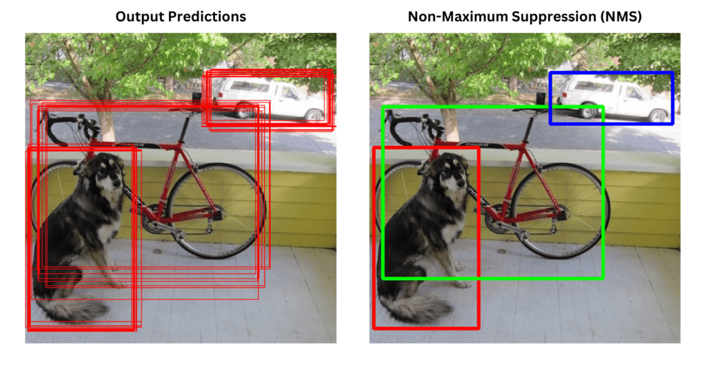
Algorithm Steps
- Sort all bounding boxes by their confidence score.
- Select the box with the highest confidence and remove it from the list.
- Compute IoU between this box and all others.
- Remove boxes with IoU above a threshold (e.g., 0.5).
- Repeat until no boxes remain.
Mathematical Intuition
Let $B_i$ be a box with score $s_i$. You iterate over all boxes and apply:
$$ \text{Keep } B_i \text{ if } IoU(B_i, B_j) < T, \forall j < i $$
Where $T$ is the suppression threshold.
Anchor Boxes
What are Anchor Boxes?
Anchor boxes (also called prior boxes) are predefined bounding boxes with different shapes and sizes. They allow object detectors to:
- Detect multiple objects in the same grid cell
- Handle aspect ratio and scale variation
Why Are They Needed?
Without anchor boxes, a single grid cell could detect only one object. But real-world scenes often contain overlapping or closely spaced objects.
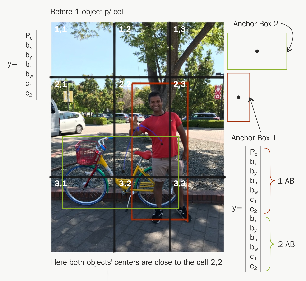
Anchor Box Design
You predefine $k$ anchor boxes per cell. Each one is defined by:
- Width $w$
- Height $h$
- Aspect ratio $r = \frac{w}{h}$
For example, in SSD:
- 3 feature maps
- 6 anchors per feature cell
- $\Rightarrow$ 8732 total anchor boxes
Output Format with Anchors
For each anchor box, the network predicts:
- $\Delta x, \Delta y$: offset from anchor center
- $\Delta w, \Delta h$: log scale changes to width and height
- Confidence score
- Class probabilities
This transforms anchor box $(x_a, y_a, w_a, h_a)$ to the predicted box $(x_p, y_p, w_p, h_p)$:
$$ x_p = x_a + w_a \cdot \Delta x \ y_p = y_a + h_a \cdot \Delta y \ w_p = w_a \cdot e^{\Delta w} \ h_p = h_a \cdot e^{\Delta h} $$
Summary
- IoU measures overlap and is used for loss/evaluation.
- Non-max suppression removes redundant boxes based on IoU.
- Anchor boxes allow detection of multiple objects at different scales/aspect ratios.
Together, these techniques form the foundation of modern object detection pipelines like YOLO, SSD, and Faster R-CNN.
Region Proposals and Semantic Segmentation: U-Net
- Region Proposals
- Semantic Segmentation
- Transpose Convolutions (Deconvolution)
- U-Net Architecture Intuition
- U-Net Architecture (Full Design)
- Summary
Region Proposals
Why Region Proposals?
Traditional object detectors like sliding windows are computationally expensive due to scanning every possible region in the image. Region Proposal methods address this by generating a small number of candidate regions likely to contain objects.
Selective Search
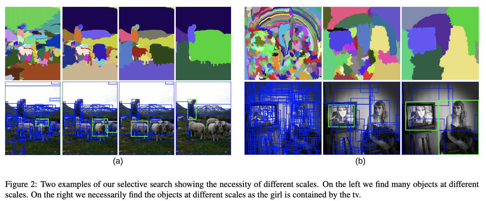
- Group similar pixels into superpixels
- Merge regions based on similarity
- Outputs ~2000 proposals per image
R-CNN Pipeline
- Use Selective Search to propose regions.
- Warp each region to a fixed size (e.g., 224x224).
- Pass through a ConvNet to extract features.
- Use SVMs for classification and regressors for bounding boxes.
Limitation: Very slow due to independent ConvNet run on each region.
Semantic Segmentation
What is Semantic Segmentation?
Semantic segmentation is the task of classifying each pixel of an image into a class label.
- Image Classification: What is in the image?
- Object Detection: Where is the object?
- Semantic Segmentation: Which pixel belongs to which class?
Applications
- Medical imaging (e.g., tumor segmentation)
- Autonomous driving (lane and pedestrian detection)
- Satellite image analysis
- Industrial defect detection
Transpose Convolutions (Deconvolution)
Motivation
In segmentation tasks, we need to upsample feature maps back to the original image size. Transpose convolutions (a.k.a. deconvolutions) help with this.
How It Works
A transpose convolution is the reverse of a normal convolution:
- While convolution reduces spatial size (downsampling),
- Transpose convolution increases it (upsampling).
Mathematical Operation
Suppose an input size of $N \times N$ and a kernel size of $k \times k$ with stride $s$.
-
Convolution output size:
$$ O = \left\lfloor \frac{N - k}{s} + 1 \right\rfloor $$
-
Transpose convolution (reverses the above): $$ O_{up} = (N - 1) \cdot s + k $$
Alternatives
- Nearest-neighbor or bilinear upsampling + 1x1 conv (cheaper, less expressive)
- Learned transpose convolutions (richer)
U-Net Architecture Intuition
Key Idea
U-Net is a fully convolutional network that consists of:
- A contracting path to capture context (downsampling)
- An expanding path to enable precise localization (upsampling)
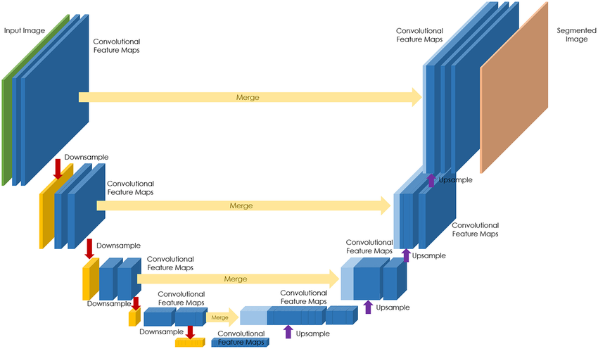
U-Net was originally designed for biomedical image segmentation but is now used in many fields.
Contracting Path (Encoder)
- Similar to standard CNN (e.g., VGG)
- Repeated 2x:
- Conv (ReLU) → Conv (ReLU) → MaxPooling
Expanding Path (Decoder)
- Transpose convolution for upsampling
- Skip connections concatenate features from encoder
Why Skip Connections?
Skip connections pass high-resolution features from encoder to decoder, enabling:
- Better boundary localization
- Preservation of fine details
U-Net Architecture (Full Design)
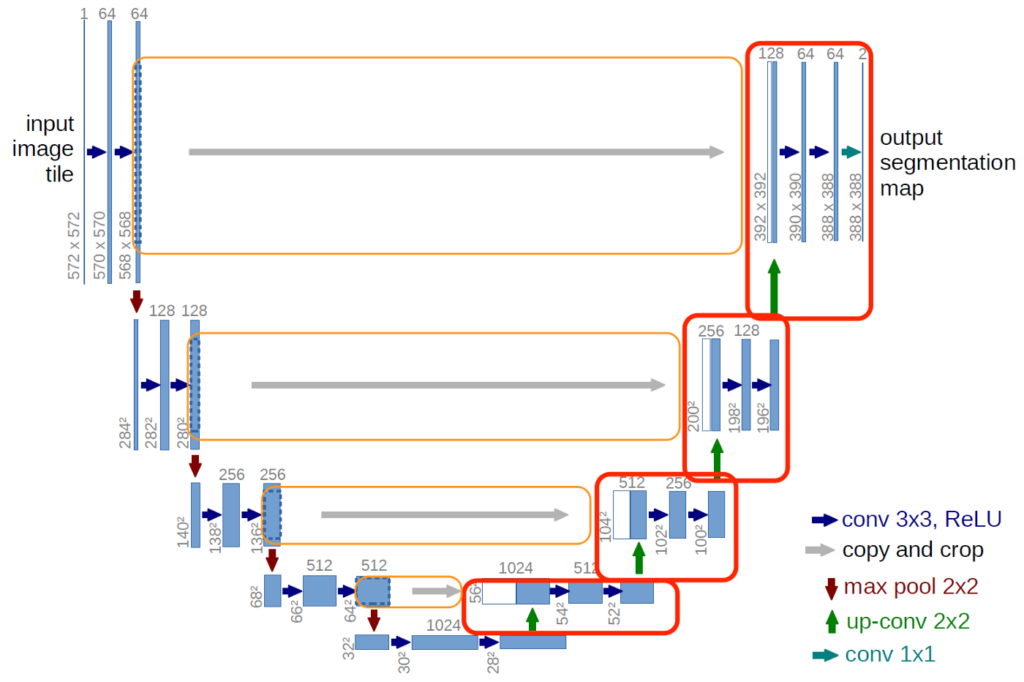
Structure Overview
- Input size: $572 \times 572$
- Each layer: two $3 \times 3$ convolutions + ReLU
- Downsampling: $2 \times 2$ max-pooling
- Upsampling: transpose convolutions
- Final output: $1 \times 1$ convolution to map to $C$ classes (per pixel)
Example Architecture
Input → Conv → Conv → Pool
      ↓             ↑
     Conv → Conv → Pool
      ↓             ↑
     Conv → Conv → Pool
      ↓             ↑
     Bottleneck     ← Skip Connections
      ↓             ↑
     Upconv → Concat → Conv → Conv
      ↓
    Output (Segmentation Map)
Loss Function
Typical loss: Pixel-wise cross-entropy loss.
$$ \mathcal{L} = - \sum_{i=1}^{H} \sum_{j=1}^{W} \sum_{c=1}^{C} y_{ij}^{(c)} \log(\hat{y}_{ij}^{(c)}) $$
Where:
- $H, W$: height and width of the image
- $C$: number of classes
- $y_{ij}^{(c)}$: ground truth indicator (1 if pixel $(i,j)$ belongs to class $c$)
- $\hat{y}_{ij}^{(c)}$: predicted probability for class $c$ at pixel $(i,j)$
Performance Metrics
- Pixel Accuracy: overall correct classification
- IoU per class: same as object detection, applied per-pixel
- Dice Coefficient: common in medical segmentation
Summary
- Region proposals are key to efficient object detection pipelines like R-CNN.
- Semantic segmentation classifies each pixel and requires upsampling layers.
- Transpose convolutions allow learned upsampling.
- U-Net combines low-level and high-level features through skip connections and is state-of-the-art for many segmentation tasks.
Face Recognition and Neural Style Transfer
What is Face Recognition?
Face recognition is the task of identifying or verifying a person’s identity using their facial features. It can be broken down into three main categories:
- Face Detection: Locate faces in an image (bounding box).
- Face Verification: Check if two faces are of the same person (1:1 comparison).
- Face Recognition/Identification: Identify a person from a database (1:N comparison).
Real-World Applications
- Smartphone unlock (Face ID)
- Security surveillance
- Online proctoring
- Social media tagging (e.g., Facebook)
One Shot Learning
Traditional classification algorithms require many training examples per class. However, in face recognition:
- We might only have one image per person.
- The task becomes: Can the model recognize a face it has seen only once?
This is known as One-Shot Learning.
Problem Setup
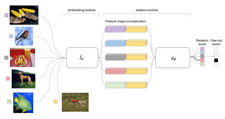
- Instead of learning to classify, the model learns similarity between pairs of images.
- A distance function is trained to return a small value for the same person, and large for different people.
Siamese Network
A Siamese Network consists of two identical ConvNets (with shared weights) that compare two inputs.
Architecture Overview
- Two inputs: $x_1$ and $x_2$
- Same CNN maps both to feature vectors $f(x_1)$ and $f(x_2)$
- A distance metric (e.g., L2 norm) is applied:
$$ d(x_1, x_2) = |f(x_1) - f(x_2)|_2^2 $$
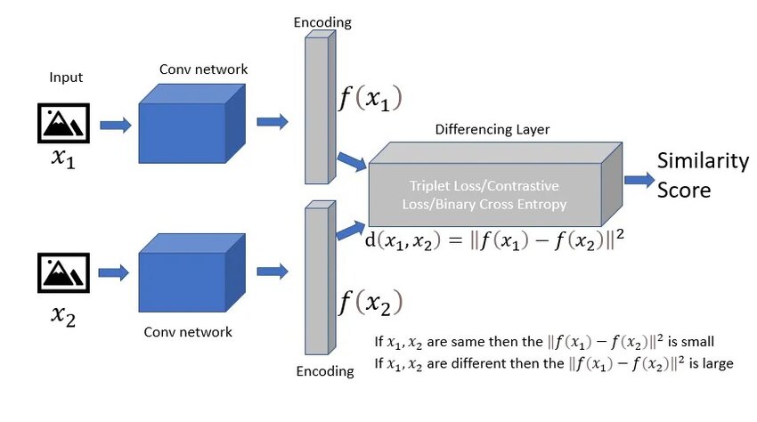
Loss Function
A contrastive loss or triplet loss is used to train the network to minimize distances for same identities and maximize for different ones.
Triplet Loss
Triplet Loss is a powerful loss function for learning embeddings. It relies on triplets:
- Anchor (A): A known image
- Positive (P): Image of the same identity
- Negative (N): Image of a different identity
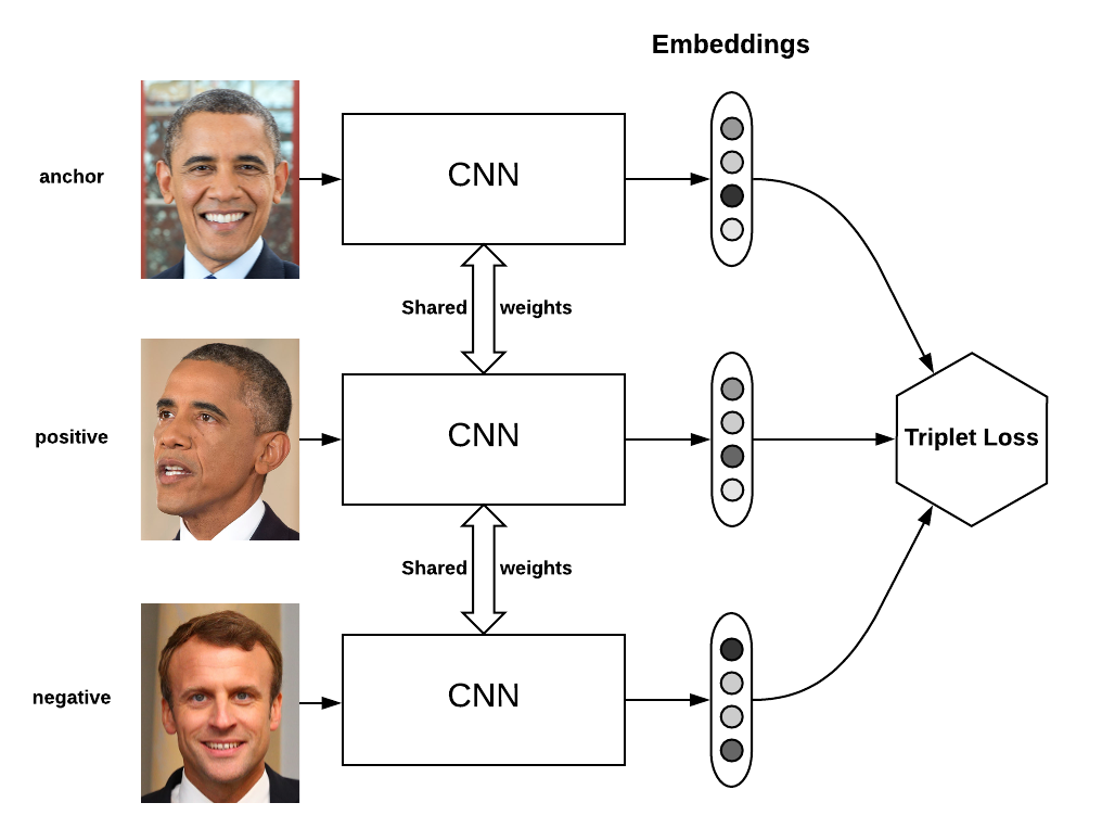
We want:
$$ |f(A) - f(P)|_2^2 + \alpha < |f(A) - f(N)|_2^2 $$
Where:
- $f(x)$ is the embedding function (ConvNet output)
- $\alpha$ is a margin to separate positive and negative pairs
Loss Function
The Triplet Loss is:
$$ \mathcal{L}(A, P, N) = \max\left(|f(A) - f(P)|_2^2 - |f(A) - f(N)|_2^2 + \alpha, 0\right) $$
Important Notes
- Semi-hard negative mining improves convergence (choose negatives that are hard but not too hard).
- Embeddings are often normalized to unit length.
Face Verification and Binary Classification
Once we have embeddings from a trained network (e.g., using triplet loss), we can perform face verification as a binary classification task.
Verification Pipeline
- Encode both face images to embeddings.
- Compute Euclidean distance or cosine similarity.
- If distance < threshold $\Rightarrow$ same person.
Threshold $\theta$ is selected based on False Positive Rate vs. True Positive Rate using ROC curve on a validation set.
What is Neural Style Transfer?
Neural Style Transfer is the task of synthesizing an image that:
- Preserves the content of a content image
- Adopts the style of a style image
Leverage a pre-trained ConvNet (like VGG19) to extract content and style representations.
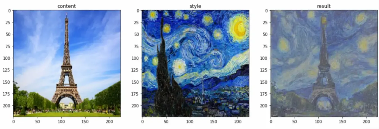
Let:
- $C$ be the content image
- $S$ be the style image
- $G$ be the generated image
Then we optimize $G$ to minimize a cost function:
$$ J(G) = \alpha J_{content}(C, G) + \beta J_{style}(S, G) $$
What are Deep ConvNets Learning?
Deep ConvNets learn hierarchical representations:

- Early layers: edges, colors, textures
- Mid layers: shapes, motifs
- Later layers: object-level concepts
In NST, content is encoded in deeper layers, style in shallower layers.
Cost Function
The total cost is:
$$ J(G) = \alpha J_{content}(C, G) + \beta J_{style}(S, G) $$
Where:
- $\alpha$: weight for content preservation
- $\beta$: weight for style transfer
- Typically: $\alpha = 1$, $\beta = 10^3$ to $10^4$
Content Cost Function
Let $a^{l}$ and $a^{l}$ be activations at layer $l$ for the content and generated images.
Then content cost is:
$$ J_{content}(C, G) = \frac{1}{2} |a^{l} - a^{l}|_2^2 $$
Use a deeper layer (e.g., conv4_2) for this.
Style Cost Function
Style is captured by correlations between feature maps using a Gram matrix.
Let $a^{l}$ be the activations at layer $l$ for style image. Compute Gram matrix:
$$ G_{ij}^{[l]} = \sum_k a_{ik}^{[l]} a_{jk}^{[l]} $$
Style cost is:
$$ J_{style}^{[l]}(S, G) = \frac{1}{(2n_H n_W n_C)^2} |G^{l} - G^{l}|_F^2 $$
Then sum over multiple layers:
$$ J_{style}(S, G) = \sum_l \lambda^{[l]} J_{style}^{[l]}(S, G) $$
1D and 3D Generalizations
1D Generalization
Neural style transfer principles can be applied to audio signals:
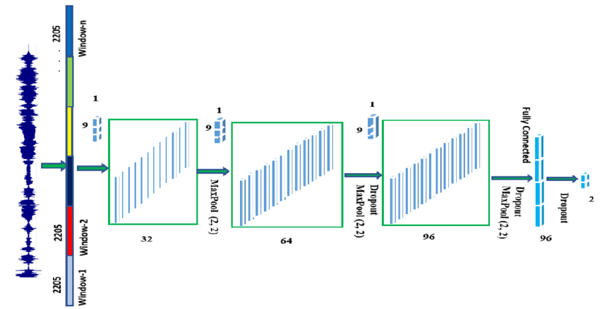
- 1D convolution over waveform
- Preserve temporal content, apply style of another sound
3D Generalization
Applied to volumetric data such as:
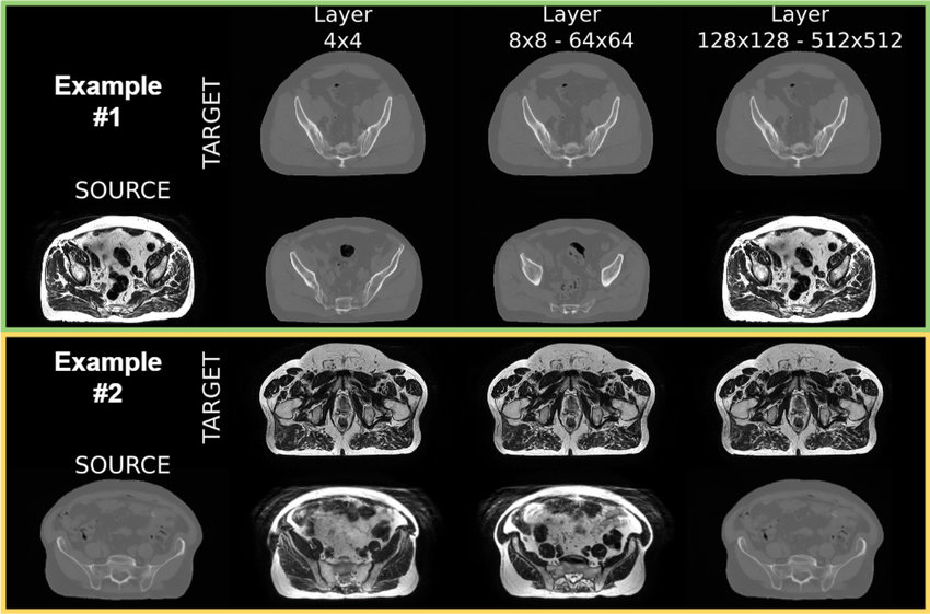
- 3D MRI scans
- 3D point clouds
- Transfer spatial styles across 3D volumes
These require 3D convolutional layers and custom Gram matrix calculations.
Summary
- Face Recognition uses embedding learning (Triplet loss, Siamese networks).
- One-shot learning enables models to generalize with limited data.
- Neural Style Transfer uses a pre-trained CNN to blend content and style images using a combination of content/style loss.
- Both applications showcase the expressive power of deep convolutional networks beyond classic classification.
Recurrent Neural Networks (RNNs)
- Why Sequence Models?
- Notation
- Recurrent Neural Network Model
- Backpropagation Through Time
- Different Types of RNNs
- Language Model and Sequence Generation
- Sampling Novel Sequences
- Vanishing Gradients with RNNs
- Gated Recurrent Unit (GRU)
- Long Short-Term Memory (LSTM)
- Bidirectional RNN
- Deep RNNs
Why Sequence Models?
Sequence models are used when the input and/or output is sequential. For example:
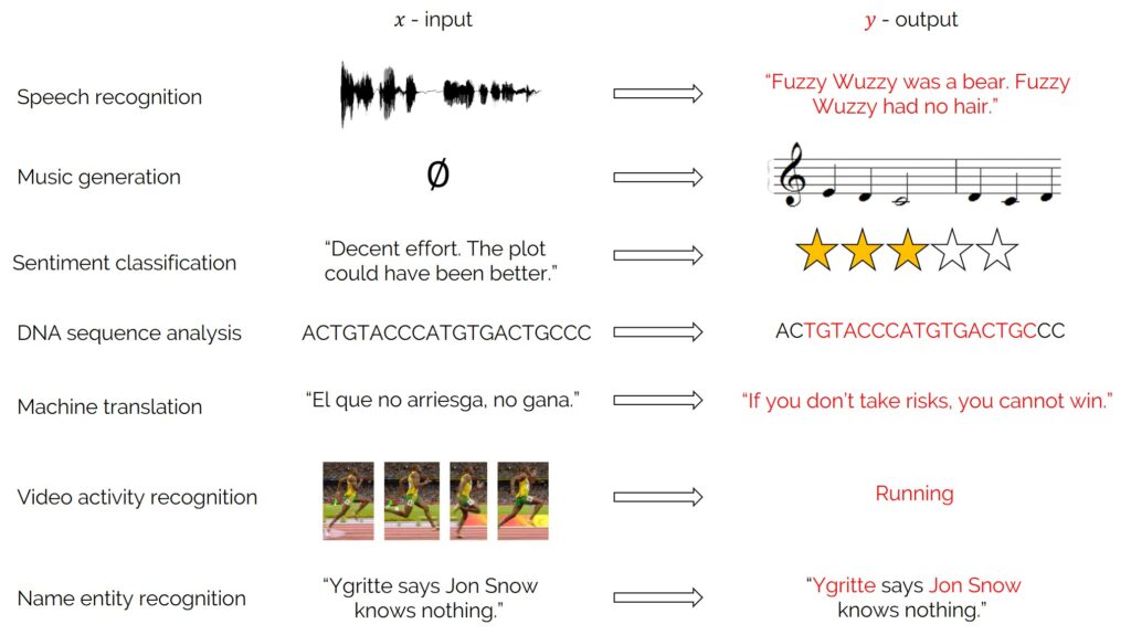
They model dependencies over time or sequence positions, which standard feedforward neural networks cannot do efficiently.
Notation
- $x^{(t)}$: input at time step $t$
- $y^{(t)}$: output at time step $t$
- $a^{(t)}$: hidden state at time step $t$
- $\hat{y}^{(t)}$: predicted output at time step $t$
- $T$: sequence length
Recurrent Neural Network Model
The RNN computes:
- $a^{(t)} = anh(W_{aa}a^{(t-1)} + W_{ax}x^{(t)} + b_a)$
- $\hat{y}^{(t)} = ext{softmax}(W_{ya}a^{(t)} + b_y)$
RNNs share parameters across time, allowing generalization to different sequence lengths.
Backpropagation Through Time
To train RNNs, we use backpropagation through time (BPTT):
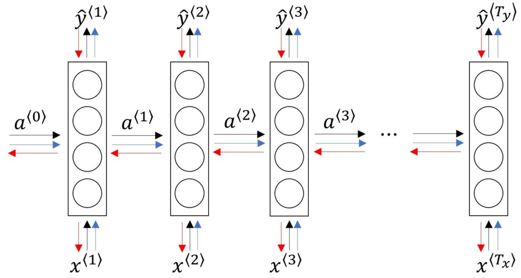
- Unroll the RNN for $T$ steps
- Compute loss and gradients across all time steps
- Apply chain rule for gradients through time dependencies
Different Types of RNNs
- Many-to-Many: sequence input and sequence output (e.g., machine translation)
- Many-to-One: sequence input, single output (e.g., sentiment analysis)
- One-to-Many: single input, sequence output (e.g., image captioning)
Language Model and Sequence Generation
Language models predict the next word given a sequence:
- $P(y^{(t)} | y^{(1)}, …, y^{(t-1)})$
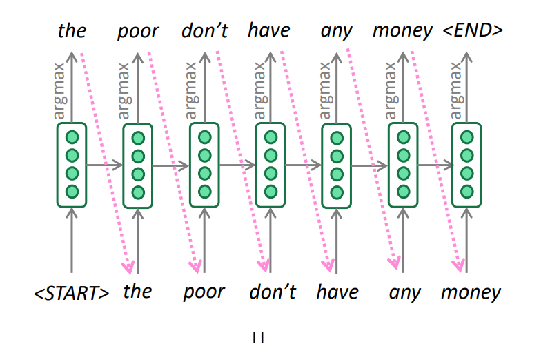
Training: minimize cross-entropy loss between predicted and actual next words.
Sampling Novel Sequences
- Start with a seed (e.g.,
) - Sample $y^{(1)}$, feed it back
- Continue until
or max length
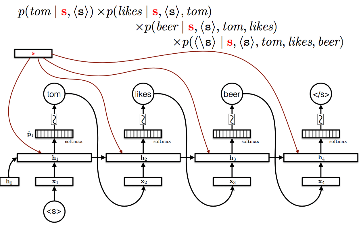
Sampling temperature can control randomness:
- Low temperature = conservative (likely choices)
- High temperature = creative (diverse outputs)
Vanishing Gradients with RNNs
One of the fundamental challenges in training RNNs is the vanishing gradient problem, especially when modeling long-term dependencies.
When computing gradients using Backpropagation Through Time (BPTT), the gradients at earlier time steps are affected by the repeated multiplication of small values (from derivatives of activation functions like tanh or sigmoid). This leads to:
- Gradients becoming very small (vanish): weights are barely updated for earlier time steps
- Gradients becoming very large (explode): instability and divergence in training
Intuition with Example:
Consider a sequence: “I grew up in France… I speak fluent ___”
The model needs to learn that the word “French” depends on the context word “France” seen many time steps earlier. If the gradient shrinks too much over those steps, the model fails to learn this dependency.
Consequences:
- Short-term dependencies are learned effectively.
- Long-term dependencies are often lost.
Gated Recurrent Unit (GRU)
Why do we need GRUs?
Traditional RNNs struggle with learning long-term dependencies due to the vanishing gradient problem. As sequences grow longer, the gradients used during backpropagation either shrink or explode, making it hard for the network to retain information over time.
GRUs are designed to solve this by introducing gating mechanisms that control what information should be remembered, updated, or forgotten. These gates make the network more efficient at learning dependencies in long sequences.
GRU introduces gates to control information flow:
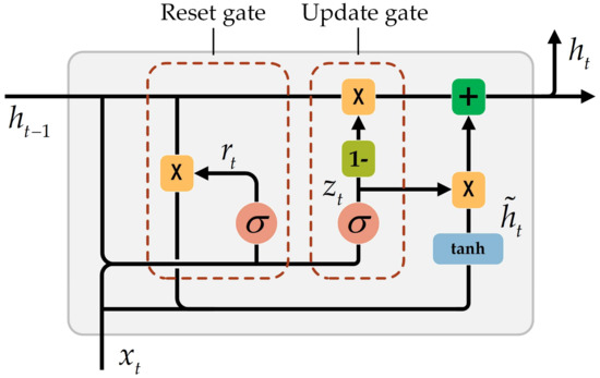
A GRU has two main gates:
-
Update Gate ($z$):
-
Determines how much of the previous memory to keep.
-
If z ≈ 1, it keeps the old memory.
-
If z ≈ 0, it updates with new information.
-
-
Reset Gate ($r$):
-
Controls how much of the previous state should be ignored.
-
Helps in deciding whether to forget the old state when generating the new memory.
-
Equations:
- $z^{(t)} = \sigma(W_zx^{(t)} + U_za^{(t-1)} + b_z)$
- $r^{(t)} = \sigma(W_rx^{(t)} + U_ra^{(t-1)} + b_r)$
- $\tilde{a}^{(t)} = \tanh(Wx^{(t)} + U(r^{(t)} \ast a^{(t-1)}) + b)$
- $a^{(t)} = (1 - z^{(t)}) * a^{(t-1)} + z^{(t)} * \tilde{a}^{(t)}$
GRU vs Traditional RNN
| Feature | RNN | GRU |
|---|---|---|
| Memory control | None | Yes (update/reset gates) |
| Vanishing gradients | Common | Less frequent |
| Parameter efficiency | Fewer params | More, but fewer than LSTM |
| Training speed | Fast | Slower than RNN, faster than LSTM |
Example: Sequence with Context
Imagine trying to classify the sentiment of the sentence:
“The movie was terrible… but the ending was amazing.”
- A vanilla RNN might forget the earlier “terrible” and overly weight the “amazing”, resulting in an incorrect positive classification.
- A GRU, however, can learn to retain both sentiments and give a more balanced representation by preserving long-term context.
Long Short-Term Memory (LSTM)
Why Do We Need LSTM?
Traditional RNNs struggle with long-term dependencies due to vanishing gradients, which hinder learning over long sequences.
To solve this, LSTMs introduce memory cells and gates that help preserve and regulate information across time steps.
LSTM Architecture Intuition
LSTM cells introduce three gates to control information:
- Forget Gate: Decides what information to throw away from the cell state.
- Input Gate: Decides which new information should be stored in the cell state.
- Output Gate: Decides what to output based on the cell state.
This gating mechanism allows the model to retain relevant information over long durations while discarding unnecessary data.
LSTM Cell: Step-by-Step
Let’s break down an LSTM cell computation for a single time step $ t $. Let:
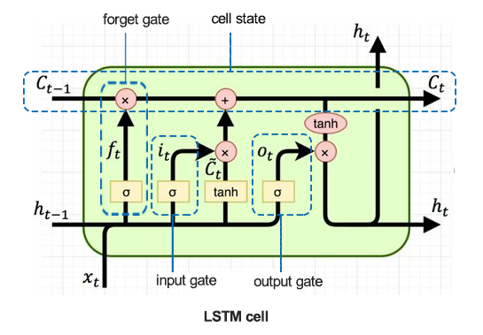
- $ x^{\langle t \rangle} $: input at time $ t $
- $ a^{\langle t-1 \rangle} $: hidden state from previous step
- $ c^{\langle t-1 \rangle} $: cell state from previous step
Then, the LSTM performs the following operations:
-
Forget Gate $ f^{\langle t \rangle} $:
$$ f^{\langle t \rangle} = \sigma(W_f \cdot [a^{\langle t-1 \rangle}, x^{\langle t \rangle}] + b_f) $$
Decides what to forget from the previous cell state.
-
Input Gate $ i^{\langle t \rangle} $ and Candidate Values $ \tilde{c}^{\langle t \rangle} $:
$$ i^{\langle t \rangle} = \sigma(W_i \cdot [a^{\langle t-1 \rangle}, x^{\langle t \rangle}] + b_i) $$
$$ \tilde{c}^{\langle t \rangle} = \tanh(W_c \cdot [a^{\langle t-1 \rangle}, x^{\langle t \rangle}] + b_c) $$
Determines what new information to add to the cell state.
-
Update Cell State:
$$ c^{\langle t \rangle} = f^{\langle t \rangle} - c^{\langle t-1 \rangle} + i^{\langle t \rangle} - \tilde{c}^{\langle t \rangle} $$
-
Output Gate $ o^{\langle t \rangle} $ and Hidden State $ a^{\langle t \rangle} $: $$ o^{\langle t \rangle} = \sigma(W_o \cdot [a^{\langle t-1 \rangle}, x^{\langle t \rangle}] + b_o) $$ $$ a^{\langle t \rangle} = o^{\langle t \rangle} * \tanh(c^{\langle t \rangle}) $$
Example: Comparing RNN and LSTM
Suppose we want to predict the next word in a sentence. Let’s compare:
RNN:
- Struggles to maintain context when sentences are long.
- For example:
"The cat, which was chased by the dog, ran up the..." → "tree"→ the subject “cat” may be forgotten.
LSTM:
- Maintains the context of “the cat” and successfully predicts
"tree".
| Feature | RNN | LSTM |
|---|---|---|
| Handles Long-Term Dependencies | ❌ | ✅ |
| Vanishing Gradient Resistant | ❌ | ✅ |
| Uses Gates | ❌ | ✅ (Forget, Input, Output) |
| Computational Complexity | Low | Higher, but more expressive |
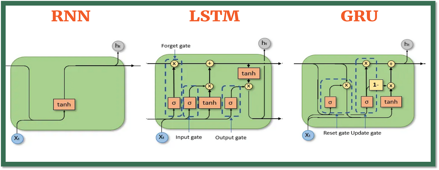
LSTMs are widely used in natural language processing, speech recognition, time series forecasting, and anywhere long-term memory is crucial.
Bidirectional RNN
In a standard RNN, information flows in a single direction — typically from past to future. However, in many tasks (like speech recognition or named entity recognition), context from both past and future words is useful for understanding the current input. This is where Bidirectional RNNs (BiRNNs) come in.
Why Use Bidirectional RNNs?
A Bidirectional RNN processes the input sequence in both directions with two separate hidden layers:
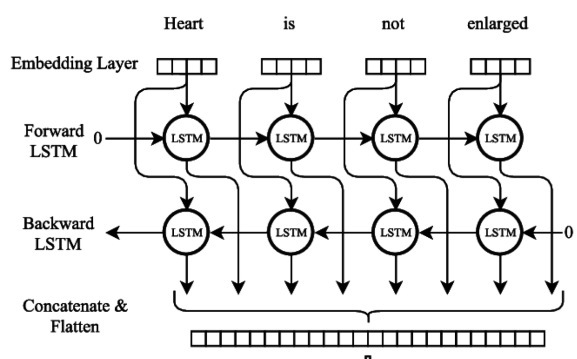
- One moves forward through time (from $x_1$ to $x_T$)
- One moves backward through time (from $x_T$ to $x_1$)
The outputs of both directions are concatenated at each time step:
$$ \overrightarrow{h}^{(t)} = \text{forward RNN output at time } t \ \overleftarrow{h}^{(t)} = \text{backward RNN output at time } t \ h^{(t)} = [\overrightarrow{h}^{(t)}; \overleftarrow{h}^{(t)}] $$
- Access to future context: Helps the model make better predictions at each time step.
- Improved performance: Especially effective in tasks where the meaning of a word depends on both previous and next words.
Imagine the sentence:
“He said he saw a bat.”
If we only process the sentence from left to right, the meaning of the word “bat” is unclear until we see the following context. A Bidirectional RNN can process both directions and better disambiguate the meaning using the full sentence context.
Applications
- Named Entity Recognition (NER)
- Part-of-Speech (POS) tagging
- Speech recognition
- Text classification
Bidirectional RNNs are often used with LSTM or GRU units to capture long-term dependencies more effectively in both directions.
Deep RNNs
Deep RNNs consist of stacking multiple recurrent layers on top of each other, allowing the network to learn hierarchical representations of sequences. By increasing the depth, the model can capture more complex temporal patterns and abstractions.
- Each layer’s output serves as input to the next recurrent layer.
- Enables learning of higher-level features across time steps.
- Can improve model capacity and expressiveness.
Challenges:
- Increased risk of overfitting due to more parameters.
- Training can be slower and more difficult due to vanishing/exploding gradients.
Applications:
- Complex sequence modeling tasks such as speech recognition, language modeling, and video analysis.
Deep RNNs are often combined with advanced units like LSTM or GRU to mitigate training difficulties and capture long-term dependencies effectively.
Natural Language Processing and Word Embeddings
- Word Representation
- Using Word Embeddings
- Properties of Word Embeddings
- Embedding Matrix
- Learning Word Embeddings
- Word2Vec
- Negative Sampling
- GloVe Word Vectors
- Sentiment Classification
- Debiasing Word Embeddings
Word Representation
In Natural Language Processing (NLP), word representation refers to how words are converted into a numerical form that a machine learning model can understand. Traditional approaches used one-hot encoding, where each word is represented by a binary vector of the vocabulary size. However, one-hot vectors suffer from high dimensionality and no semantic information.
Example:
This image shown one-hot embedding example.
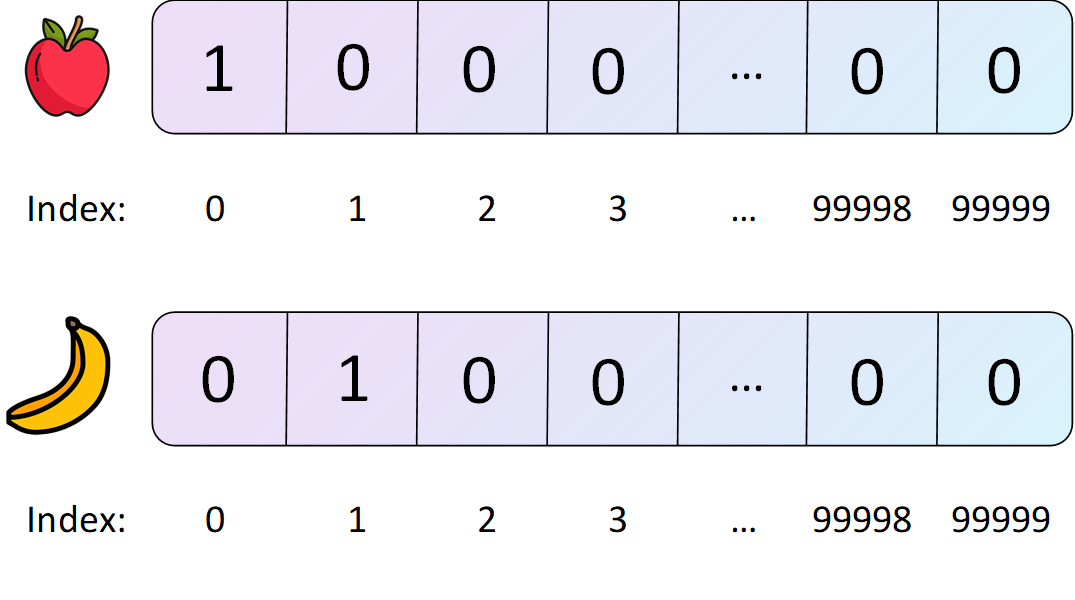
Vocabulary: ["king", "banana", "apple"]
One-hot representation of "king": [1, 0, 0]
One-hot representation of "banana": [0, 1, 0]
One-hot representation of "apple": [0, 0, 1]
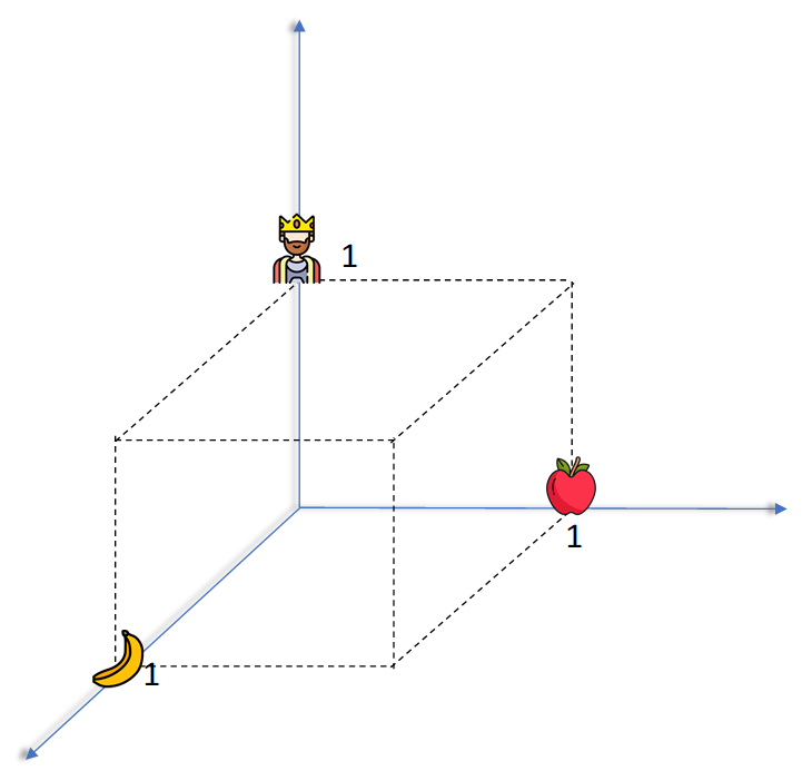
This representation doesn’t capture the relationship between “banana” and “apple” or that both are fruit. Hence, we need better methods like word embeddings.
Using Word Embeddings
Word embeddings are dense vector representations of words in a continuous vector space, where semantically similar words are mapped closer together.
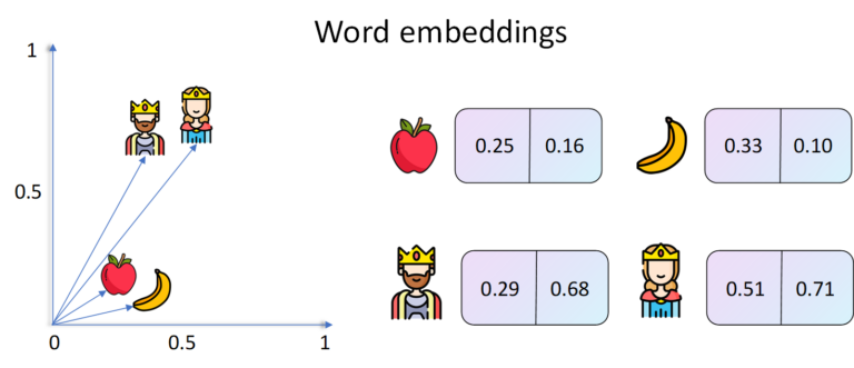
Example: A 3D visualization might show vectors such that:
- vector(“king”) - vector(“man”) + vector(“woman”) ≈ vector(“queen”)
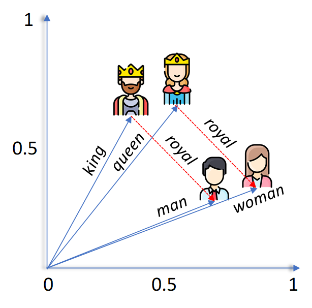
This arithmetic reflects the semantic relationship between the words, allowing machines to understand analogies.
Properties of Word Embeddings
Word embeddings exhibit fascinating properties:
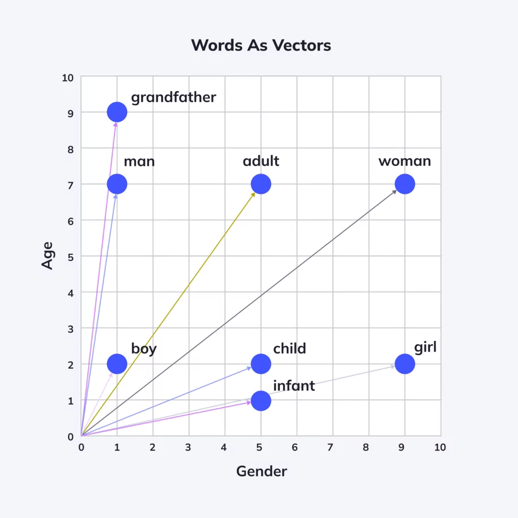
- Semantic similarity: Similar words have vectors close to each other (e.g., “good” and “great”).
- Linear substructures: Relationships can be captured with simple vector arithmetic (e.g., “Paris” - “France” + “Italy” ≈ “Rome”).
- Dimensionality reduction: Embeddings reduce high-dimensional one-hot vectors to lower-dimensional dense vectors (e.g., from 10,000 to 300 dimensions).
Embedding Matrix
An embedding matrix is a trainable matrix in a neural network where each row corresponds to a word’s vector.
Structure:
- Suppose the vocabulary size is
V = 10,000and the embedding size isN = 300. - The embedding matrix
Ewill have shape(V, N).
To retrieve the embedding of word i, simply use:
embedding_vector = E[i]
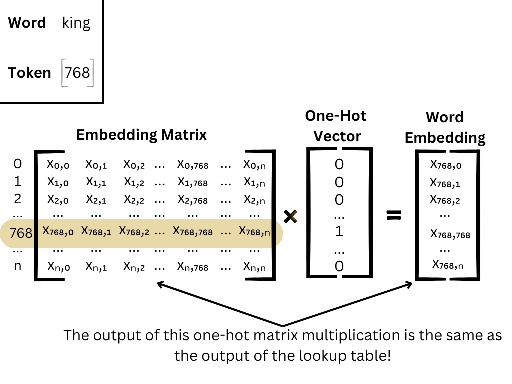
This matrix is updated during training so that embeddings capture task-specific information.
Learning Word Embeddings
Word embeddings can be learned in two ways:
- Supervised Learning: Train a model on a downstream task (e.g., sentiment classification) and update embeddings during training.
- Unsupervised Learning: Train embeddings on large text corpora to learn general-purpose representations (e.g., Word2Vec, GloVe).
Word2Vec
Word2Vec is a popular unsupervised model for learning word embeddings. It has two architectures:
Architectures: CBOW vs Skip-Gram
Word2Vec comes in two main model architectures:
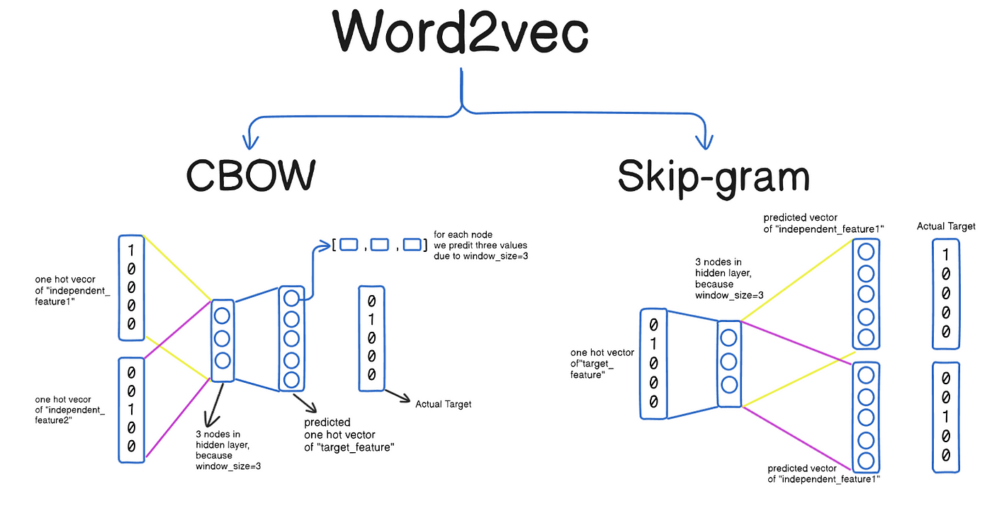
-
Continuous Bag of Words (CBOW):
Predicts the current word based on its context.
Given the surrounding words, the model tries to guess the center word.
Efficient for larger datasets and more frequent words.Example:
- Input: [“the”, “cat”, “on”, “the”, “mat”]
- Center Word: “sat”
- Context: [“the”, “cat”, “on”, “the”, “mat”]
- CBOW tries to predict “sat” from the context.
-
Skip-Gram:
Predicts surrounding context words given the current word.
Given the center word, the model tries to predict the context.
Performs well with smaller datasets and rare words.Example:
- Input: “sat”
- Target Outputs: [“the”, “cat”, “on”, “the”, “mat”]
- Skip-Gram tries to predict the surrounding words from “sat”.
How Word2Vec Learns Word Embeddings
- Word2Vec uses a shallow neural network with one hidden layer.
- The vocabulary size is
V, and the desired vector size isN. - The input layer is a one-hot vector of size
V. - The hidden layer (no activation function) has size
N. - The output layer is also of size
V, predicting a probability distribution over all words.
Steps:
- Convert the input word into a one-hot encoded vector.
- Multiply it by the input weight matrix to get the hidden layer representation.
- Multiply that by the output weight matrix to get scores for all words in the vocabulary.
- Apply softmax to produce a probability distribution.
- Update weights via backpropagation using gradient descent to minimize the loss.
Training Objective: Maximizing Log Probability
For the Skip-Gram model, the goal is to maximize the average log probability:
$$ \frac{1}{T} \sum*{t=1}^{T} \sum*{-m \leq j \leq m, j \neq 0} \log p(w_{t+j} | w_t) $$
Where:
- $ T $ is the total number of words in the corpus.
- $ m $ is the context window size.
- $ wt $ is the center word, and $ w{t+j} $ are the context words.
Computational Challenge: Softmax and Large Vocabulary
Calculating the softmax over a large vocabulary is computationally expensive. To address this, Word2Vec introduces optimization techniques such as:
- Negative Sampling
- Hierarchical Softmax
These methods significantly reduce the training time while maintaining the quality of the learned embeddings.
Example: Learning from a Sentence
Suppose the sentence is:
"The quick brown fox jumps over the lazy dog"
With a context window of size 2, for the center word “brown”, the context is [“The”, “quick”, “fox”, “jumps”].
In the Skip-Gram model, we would train the network to predict each of those context words from “brown”.
Why Word2Vec Works
Word2Vec learns useful representations because:
- It captures both syntactic and semantic relationships.
- It leverages co-occurrence statistics of words in a corpus.
- The vector space preserves many linguistic regularities.
For instance:
vec("Paris") - vec("France") + vec("Italy") ≈ vec("Rome")vec("walking") - vec("walk") + vec("swim") ≈ vec("swimming")
Applications of Word2Vec
- Text classification
- Sentiment analysis
- Named entity recognition
- Question answering
- Semantic search
- Machine translation
These embeddings can be pre-trained (e.g., on Google News) or trained on custom corpora to tailor them to specific domains (e.g., medical texts, legal documents).
Negative Sampling
In Word2Vec, instead of updating weights for all words in the vocabulary, negative sampling updates only a few:
- Pick one positive pair (word and context).
- Sample
knegative words randomly.
This improves efficiency dramatically and allows the model to scale to large corpora.
Loss function (simplified):
$$ \log(\sigma(v_c \cdot v_w)) + \sum_{j=1}^k \mathbb{E}{w_j \sim P_n(w)}[\log(\sigma(-v{w_j} \cdot v_w))] $$
Where:
v_wis the input word vectorv_cis the context vectorP_n(w)is the noise distribution
GloVe Word Vectors
GloVe (Global Vectors for Word Representation) is an alternative to Word2Vec. It constructs a co-occurrence matrix X and models the relationships between words based on their global co-occurrence statistics.
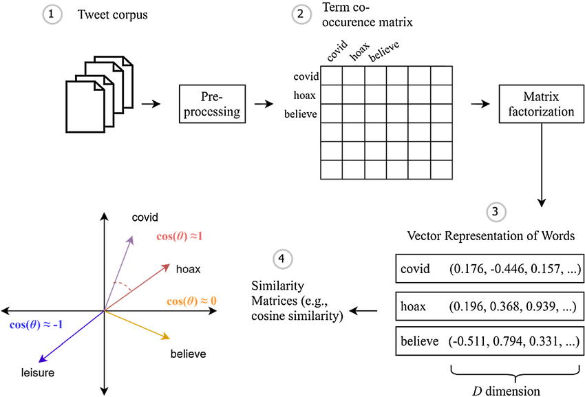
Cost function:
$$ J = \sum_{i,j=1}^{V} f(X_{ij})(w_i^T \tilde{w}_j + b_i + \tilde{b}j - \log X{ij})^2 $$
Where:
- $X_ij$ = number of times word $i$ co-occurs with word $j$
- $w_i$, $\tilde{w}_j$ = word vectors
- $b_i$, $\tilde{b}_j$ = biases
- $f(X)$ = weighting function
This approach captures both local and global word relationships.
Sentiment Classification
Word embeddings can be used as inputs to models like LSTM or CNN for tasks such as sentiment analysis.
Example workflow:
- Convert text to sequence of embeddings.
- Feed sequence into an LSTM.
- Predict a sentiment label: positive, negative, or neutral.
Embeddings help capture contextual sentiment information that traditional methods might miss.
Debiasing Word Embeddings
Word embeddings can reflect and amplify societal biases (e.g., gender bias).
Example:
- vector(“doctor”) might be closer to vector(“man”) than vector(“woman”) in biased embeddings.
Debiasing Techniques:
- Identify bias subspace: e.g., direction of gender (he-she).
- Neutralize: Make gender-neutral words (e.g., “doctor”) orthogonal to the gender direction.
- Equalize: Adjust word pairs (e.g., “man” and “woman”) to be equidistant from neutral terms.
These techniques are essential to make NLP applications fair and inclusive.
This concludes a comprehensive overview of word embeddings and their usage in natural language processing. Each concept here forms the foundation for more advanced NLP models such as Transformers and BERT.
Content
First Principles of Computer Vision
Notes taken during the First Principles of Computer Vision Specialization
by Shree K. Nayar
Columbia University
Courses
| # | Course | Status |
|---|---|---|
| 1 | Introduction to Computer Vision | ✅ |
| 2 | Imaging | ⬜ |
| 3 | Features | ⬜ |
| 4 | Reconstruction I | ⬜ |
| 5 | Reconstruction II | ⬜ |
| 6 | Perception | ⬜ |
— emreaslan —
Introduction to Computer Vision
- 1. What is Computer Vision?
- 2. The Human Visual System: Biology, Fallibility, and Ambiguity
- 3. Topics Covered: Roadmap
- 4. Global Applications: Computer Vision in the Modern World
1. What is Computer Vision?
Computer vision is not merely a subset of artificial intelligence; it is a profound multidisciplinary engineering and scientific enterprise. It bridges the physical world and symbolic understanding, drawing upon optics, signal processing, electrical engineering, and computer science.
Vision pipeline: light source → scene → camera → Vision Software produces a scene description
The fundamental challenge lies in transforming raw numerical arrays—pixel data—into a meaningful description of the 3D environment.

Raw visual input: two children showering
Same scene as a numerical pixel matrix
In this field, the definition of the mission often dictates the methodology. Below is a comparison of the three primary philosophical pillars of computer vision research:
| Perspective | Proponent | Core Philosophy |
|---|---|---|
| Vision as Emulation | David Marr | Aimed at automating human visual processes to replicate the sophistication of biological systems |
| Vision as Information Processing | Berthold Horn | Defined as the task of “inverting” image formation—mathematically walking back from a 2D projection to 3D reality |
| Vision as a Functional Tool | Takeo Kanade | Emphasizes that vision is “fun” but, more importantly, “useful,” serving as a bridge between pure research and practical application |
1.1 The “First Principles” Philosophy
While contemporary deep learning provides powerful tools, a First Principles approach—focusing on mathematical and physical underpinnings—is the prerequisite for generalizable and explainable AI. Relying on “black box” models often bypasses the structural understanding required for true innovation.
Why First Principles? Physical phenomena can be described with elegant math, making massive datasets and exhaustive training cycles unnecessary.
We prioritize these fundamentals for four reasons:
- Precision and Conciseness — Physical phenomena can often be described with elegant math, rendering massive datasets unnecessary.
- Debugging and Diagnostics — When a vision system fails, first principles provide the only rigorous framework for diagnosing the failure.
- Synthetic Data Generation — When real-world data collection is impractical or dangerous, mathematical models allow us to synthesize high-fidelity training data.
- Scientific Curiosity — The innate human drive to understand the “why” behind visual phenomena leads to breakthroughs that purely data-driven methods overlook.
2. The Human Visual System: Biology, Fallibility, and Ambiguity
Studying the human eye is a necessary starting point for designing artificial vision. Even though machines and humans often have divergent goals—qualitative navigation versus quantitative measurement—the eye provides a blueprint for efficient information reduction.
2.1 The Biological Pathway
The human visual system is a complex hierarchy designed for rapid analysis:
flowchart LR
    A["👁️ Eye & Lens<br/><i>Primary optical stage</i>"] --> B["🧬 Retina<br/><i>Early processing + data reduction</i>"]
    B --> C["🔌 Optic Nerve<br/><i>High-speed conduit</i>"]
    C --> D["🧠 LGN<br/><i>Relay station, directs to regions</i>"]
    D --> E["🎯 Visual Cortex<br/><i>Shape, color, motion, texture</i>"]

    style A fill:#1a1a2e,stroke:#e94560,color:#fff
    style B fill:#16213e,stroke:#e94560,color:#fff
    style C fill:#0f3460,stroke:#e94560,color:#fff
    style D fill:#1a1a2e,stroke:#e94560,color:#fff
    style E fill:#16213e,stroke:#e94560,color:#fff
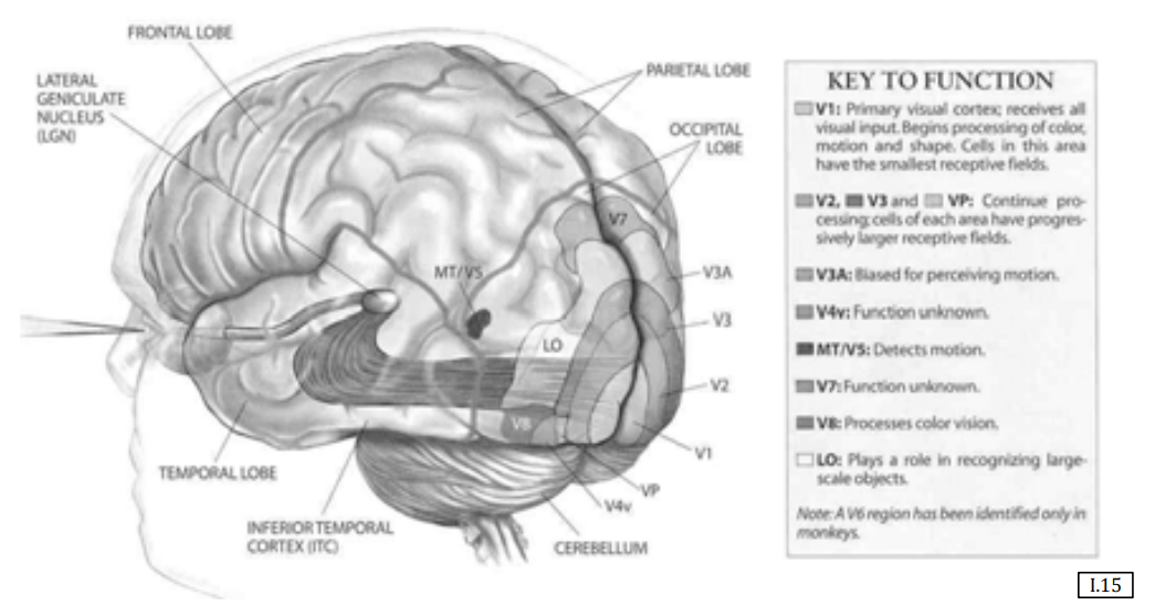
Biological vision pathway: retina → LGN → visual cortex (V1, V2, MT/V5, V8)
2.2 Qualitative vs. Quantitative Vision
As engineers, we must recognize that human vision is a qualitative system, whereas factory automation, medical imaging, and robotics require quantitative precision. A human can recognize a face instantly but cannot measure the length of a component to the nearest millimeter. For tasks requiring extreme reliability, emulating human biology is often the “wrong” goal; machines must provide the measurable accuracy that biological systems lack.
2.3 Case Studies in Visual Illusions
Human vision is more fallible than it appears, often relying on internal assumptions to resolve ambiguity.
Example — Dongary Wave Illusion: The static leaf pattern below appears to shimmer or move due to involuntary micro-saccades of the eye.
Static leaf pattern that produces a perception of motion — the Dongary Wave illusion
| Illusion | What It Reveals |
|---|---|
| Fraser’s Spiral | Concentric circles misinterpreted as a spiral |
| Adelson’s Checker Shadow | Brain compensates for illumination — two identical gray patches look different |
| Dongary Wave | Perceived motion from a static image due to involuntary eye movements |
| Ames Room | Perspective and relative size create an illusion where people appear to grow or shrink |
| Necker Cube / Faces vs. Vase | A single 2D image supports multiple 3D or symbolic interpretations |
| The Crater Illusion | The “lighting from above” assumption — flipping a mound makes it appear as a crater |
| Kanizsa Triangle | The brain “fills in” data (thinking) rather than just processing pixels (seeing) |
Key Insight: While humans think through their visual experiences, machines must first learn to calculate through the rigorous lens of radiometry and geometry.
3. Topics Covered: Roadmap
This specialization covers the entire pipeline — from pixels to perception — organized into six modules:
flowchart TB
    subgraph Foundations["🟦 Foundations"]
        direction TB
        A["Introduction<br/><i>What is CV, human vision</i>"]
        B["Imaging<br/><i>Formation, sensors, processing</i>"]
    end

    subgraph Features["🟧 Features & 2D"]
        C["Features<br/><i>Edges, SIFT, stitching, faces</i>"]
    end

    subgraph Reconstruction["🟩 3D Reconstruction"]
        D["Reconstruction I<br/><i>Radiometry, photometric stereo</i>"]
        E["Reconstruction II<br/><i>Stereo, optical flow, SfM</i>"]
    end

    subgraph Perception["🟥 Perception"]
        F["Perception<br/><i>Tracking, segmentation, NN</i>"]
    end

    A --> B --> C --> D --> E --> F

    style A fill:#1a1a2e,stroke:#4cc9f0,color:#fff
    style B fill:#1a1a2e,stroke:#4cc9f0,color:#fff
    style C fill:#1a1a2e,stroke:#f72585,color:#fff
    style D fill:#1a1a2e,stroke:#06d6a0,color:#fff
    style E fill:#1a1a2e,stroke:#06d6a0,color:#fff
    style F fill:#1a1a2e,stroke:#e94560,color:#fff
    style Foundations fill:transparent,stroke:#4cc9f0,color:#4cc9f0
    style Features fill:transparent,stroke:#f72585,color:#f72585
    style Reconstruction fill:transparent,stroke:#06d6a0,color:#06d6a0
    style Perception fill:transparent,stroke:#e94560,color:#e94560
Module Breakdown
| # | Module | Focus |
|---|---|---|
| 1 | Imaging | Image formation, sensors, binary images, image processing (convolution, Fourier) |
| 2 | Features | Edge/boundary detection, SIFT, image stitching, face detection |
| 3 | Reconstruction I | Radiometry, photometric stereo, shape from shading, depth from defocus |
| 4 | Reconstruction II | Camera calibration, stereo, optical flow, structure from motion |
| 5 | Perception | Object tracking, segmentation, appearance matching, neural networks |
4. Global Applications: Computer Vision in the Modern World
Vision has evolved from a laboratory curiosity into a thriving global industry across diverse sectors.
| Domain | Applications |
|---|---|
| Industrial / Efficiency | Factory automation, high-speed visual inspection, OCR for license plates and postal scanning |
| Security / Identity | Biometrics using iris patterns (as unique as DNA), robust face recognition |
| Consumer Tech | Optical mice (mini-vision systems), gaming (Kinect / PlayStation), AR (Snapchat 3D mesh filters) |
| Intelligent Marketing | Vending machines detecting customer demographics (age/gender) to display targeted products |
| Visual Search | Instant identification of monuments and objects via mobile devices |
| Advanced Mobility | Driverless cars using sensor fusion, Mars Rover terrain mapping |
| Creative / Medical | Motion capture for cinema, medical diagnostics (X-ray, MRI, ultrasound) |
Hoş Geldiniz
Derin Öğrenme Notları
Deep Learning Specialization kapsamında alınan notlar
Andrew Ng & Eddy Shyu tarafından
Stanford Üniversitesi & DeepLearning.AI
İşlenen Dersler
| # | Ders | Odak |
|---|---|---|
| 1 | Sinir Ağları ve Derin Öğrenme | Lojistik regresyon sinir ağı olarak, sığ & derin ağlar, ileri/geri yayılım |
| 2 | Derin Sinir Ağlarını Geliştirme | Hiperparametre ayarı, düzenlileştirme (Dropout, BatchNorm), optimizasyon (Momentum, Adam), Xavier/He başlatma |
| 3 | Makine Öğrenmesi Projelerini Yapılandırma | Train/dev/test ayrımı, hata analizi, transfer öğrenmesi, uçtan uca derin öğrenme |
| 4 | Konvolüsyonel Sinir Ağları | CNNs, kenar tespiti, klasik & modern mimariler (LeNet, AlexNet, VGG, ResNet, Inception, MobileNet, EfficientNet), nesne tespiti (YOLO), yüz tanıma (FaceNet, Siamese), neural style transfer, U-Net |
| 5 | Sequence Modelleri | RNNs, GRUs, LSTMs, kelime gömmeleri (Word2Vec, GloVe), dikkat mekanizması, Transformer, konuşma tanıma, müzik sentezi, makine çevirisi, sohbet robotları |
— emreaslan —
İçerik
Hoş geldiniz — Machine Learning notları.
∴
Machine Learning Specialization kursunu tamamlarken aldığım detaylı notlar — temel kavramlardan ileri algoritmalara, her konu kendi cümlelerimle açıklanmış ve kod örnekleriyle pekiştirilmiş.
Stanford Üniversitesi & DeepLearning.AI
— emreaslan —
Denetimli ve Denetimsiz Makine Öğrenmesi (Supervised and Unsupervised Machine Learning)
Giriş (Introduction)
Makine öğrenmesi (machine learning), yapay zekânın bir dalı olup sistemlerin açık bir şekilde programlanmadan öğrenmesine, tahminler yapmasına veya kararlar almasına olanak tanır. İki ana makine öğrenmesi türü Denetimli Öğrenme (Supervised Learning) ve Denetimsiz Öğrenmedir (Unsupervised Learning). Aşağıda, bu iki türün özelliklerini, alt alanlarını ve görsel bir temsilini bulabilirsiniz.
graph TD
    A[Makine Öğrenmesi] --> B[Denetimli Öğrenme]
    A --> C[Denetimsiz Öğrenme]
    B --> D[Regresyon]
    B --> E[Sınıflandırma]
    C --> F[Kümeleme]
    C --> G[Birliktelik]
    C --> H[Boyut İndirgeme]
Denetimli Öğrenme (Supervised Learning)
Denetimli öğrenme, modelin etiketlenmiş veriler (labeled data) üzerinde eğitildiği bir makine öğrenmesi türüdür. Etiketlenmiş veri, her girdi için karşılık gelen bir çıktının (veya hedefin) önceden sağlanmış olduğu anlamına gelir. Modelin amacı, girdiler ve çıktılar arasındaki ilişkiyi öğrenerek yeni, görülmemiş veriler için tahminler yapabilmektir.
Temel Özellikler (Key Characteristics)
- Girdi ve Çıktı: Eğitim verisi, hem girdi özelliklerini (X) hem de hedef etiketleri (Y) içerir.
- Amaç: Belirli bir girdi (X) için çıktıyı (Y) tahmin etmek.
Alt Alanlar (Subfields)
- Regresyon (Regression): Sürekli değerlerin tahmin edilmesi (örneğin, daire büyüklüğüne göre kira fiyatlarının tahmin edilmesi).
- Sınıflandırma (Classification): Girdilerin ayrık kategorilere atanması (örneğin, kanserin iyi huylu veya kötü huylu olarak teşhis edilmesi).
Örnek: Regresyon (Regression)
- Senaryo: Daire büyüklüğüne (m²) göre kira fiyatlarının tahmin edilmesi.
- Detaylar:
- Girdi özellikleri (X): Daire büyüklüğü, oda sayısı, mahalle vb.
- Hedef değişken (Y): Kira fiyatı (örneğin, aylık $).
- Modelin Görevi: Daire özellikleri ile kira fiyatları arasındaki ilişkiyi öğrenmek ve yeni bir daire için kira fiyatını tahmin etmek.

Örnek: Sınıflandırma (Classification)
- Senaryo: Kanser teşhisi (örneğin, iyi huylu veya kötü huylu tümör).
- Detaylar:
- Girdi özellikleri (X): Tümör boyutu, doku, hücre şekli gibi ölçümler.
- Hedef değişken (Y): Sınıf etiketi (örneğin, “İyi Huylu” veya “Kötü Huylu”).
- Modelin Görevi: Girdi özelliklerine dayanarak yeni bir tümörü iyi huylu veya kötü huylu olarak sınıflandırmak.

Denetimsiz Öğrenme (Unsupervised Learning)
Denetimsiz öğrenme, etiketlenmemiş veriler (unlabeled data) ile ilgilenir. Model, önceden tanımlanmış herhangi bir etiket veya hedef olmadan veri içindeki örüntüleri, yapıları veya ilişkileri bulmaya çalışır. Genellikle keşifsel veri analizi (exploratory data analysis) için kullanılır.
Temel Özellikler (Key Characteristics)
- Yalnızca Girdi: Veri, yalnızca girdi özelliklerini (X) içerir, hedef etiketleri (Y) yoktur.
- Amaç: Verideki gizli örüntüleri veya gruplaşmaları keşfetmek.
Alt Alanlar (Subfields)
- Kümeleme (Clustering): Benzer veri noktalarını kümeler halinde gruplama (örneğin, müşteri segmentasyonu).
- Boyut İndirgeme (Dimensionality Reduction): Önemli bilgileri koruyarak veri setindeki özellik sayısını azaltma (örneğin, PCA).
- Birliktelik (Association): Büyük veri setlerinde değişkenler arasındaki ilişkileri veya birliktelikleri keşfetme (örneğin, sepet analizi).
Örnek: Kümeleme (Clustering)
- Senaryo: Hedefli pazarlama için müşterilerin gruplandırılması.
- Detaylar:
- Girdi özellikleri (X): Müşteri yaşı, geliri, satın alma geçmişi, konumu vb.
- Önceden tanımlanmış etiketler (Y) yoktur.
- Modelin Görevi: Müşteri kümelerini belirlemek (örneğin, “Yüksek harcamacılar,” “Bütçe bilincine sahip alıcılar”).

Örnek: Boyut İndirgeme (Dimensionality Reduction)
- Senaryo: Yüksek boyutlu verilerin görselleştirilmesi.
- Detaylar:
- 100’den fazla özelliğe sahip bir veri setiniz olduğunu düşünün (örneğin, bir fabrikadan alınan sensör verileri).
- Boyut indirgeme (örneğin, PCA), daha kolay görselleştirme için veriyi 2B veya 3B’ye indirgemeye yardımcı olur.
- Modelin Görevi: Karmaşıklığı azaltırken verinin önemli yapısını korumak.

Örnek: Birliktelik (Association)
- Senaryo: Ürün birlikteliklerini belirlemek için sepet analizi (market basket analysis).
- Detaylar:
- Girdi özellikleri (X): Birlikte satın alınan ürünleri gösteren işlem verileri.
- Önceden tanımlanmış etiketler (Y) yoktur.
- Modelin Görevi: “Bir müşteri ekmek alıyorsa, tereyağı alma olasılığı yüksektir” gibi kurallar belirlemek.
- Kullanım Alanı: Öneri sistemleri, envanter planlaması.

Karşılaştırma Tablosu (Comparison Table)
| Özellik | Denetimli Öğrenme | Denetimsiz Öğrenme |
|---|---|---|
| Veri Türü | Etiketlenmiş veri (X, Y) | Etiketlenmemiş veri (yalnızca X) |
| Amaç | Sonuçları tahmin etmek | Örüntüler veya yapılar bulmak |
| Temel Teknikler | Regresyon, Sınıflandırma | Kümeleme, Boyut İndirgeme, Birliktelik |
| Örnekler | Dolandırıcılık tespiti, Hisse senedi fiyat tahmini | Pazar segmentasyonu, Görüntü sıkıştırma |
Anahtar Çıkarımlar (Key Takeaways)
- Denetimli Öğrenme, etiketlenmiş veri gerektirir ve regresyon ile sınıflandırma gibi tahmin görevlerinde yaygın olarak kullanılır.
- Denetimsiz Öğrenme, etiketlenmemiş verilerle çalışır ve kümeleme veya boyut indirgeme yoluyla gizli örüntüleri bulmaya odaklanır.
- Her tekniğin belirli uygulamaları vardır ve probleme ile mevcut veriye göre seçilir.
- Lineer Regresyon ve Maliyet Fonksiyonu (Linear Regression and Cost Function)
Lineer Regresyon ve Maliyet Fonksiyonu (Linear Regression and Cost Function)
1. Giriş (Introduction)
Lineer regresyon (linear regression), makine öğrenimindeki temel algoritmalardan biridir. Özellikle girdi ve çıktı değişkenleri arasındaki ilişkinin doğrusal olduğu varsayıldığında, tahmine dayalı modelleme (predictive modeling) için yaygın olarak kullanılır. Temel amaç, tahmin edilen değerler ile gerçek değerler arasındaki hatayı en aza indiren en uygun doğruyu bulmaktır.
Neden Lineer Regresyon?
Lineer regresyon, birçok gerçek dünya uygulaması için basit ancak güçlüdür. Bazı yaygın kullanım alanları şunlardır:
- Ev fiyatlarını tahmin etmek — büyüklük, oda sayısı ve konum gibi özelliklere dayanarak.
- Maaşları tahmin etmek — deneyim, eğitim seviyesi ve sektöre göre.
- Trendleri anlamak — finans, sağlık ve ekonomi gibi çeşitli alanlarda.
Gerçek Dünya Örneği: Konut Fiyatları
Ev büyüklüğüne (metrekare cinsinden) dayanarak ev fiyatlarını tahmin etmeyi düşünelim. Basit bir doğrusal ilişki varsayılabilir: daha büyük evler daha yüksek fiyatlara sahip olma eğilimindedir. Bu varsayım, lineer regresyon modelimizin temelidir.

2. Matematiksel Gösterim (Mathematical Representation)
Basit bir lineer regresyon modeli, girdi $x$ (metrekare cinsinden ev büyüklüğü) ile çıktı $y$ (ev fiyatı) arasında doğrusal bir ilişki olduğunu varsayar. Şu şekilde gösterilir:
$$ h_θ(x) = \theta_0 + \theta_1 x $$
burada:
- $h_θ(x) $ tahmin edilen ev fiyatıdır.
- $ \theta_0 $ (kesim noktası - intercept) ve $\theta_1 $ (eğim - slope) modelin parametreleridir.
- $x$ ev büyüklüğüdür.
- $y$ gerçek ev fiyatıdır.
2.1 Lineer Modeli Anlamak
Peki bu denklem gerçekte ne anlama geliyor?
-
$\theta_0$ (kesim noktası - intercept): Büyüklüğü 0 m² olduğunda bir evin fiyatı.
-
$\theta_1$ (eğim - slope): Her ilave metrekare için ev fiyatındaki artış.
Örneğin, eğer:
-
$\theta_0 = 50,000$ ve $\theta_1 = 300$ ise,
-
100 m²’lik bir evin maliyeti: $ h_θ(100) = 50000 + 300 \cdot 100 = 80000 $
-
200 m²’lik bir evin maliyeti: $ h_θ(200) = 50000 + 300 \cdot 200 = 110000 $
Bu ilişkiyi bir regresyon doğrusu kullanarak görselleştirebiliriz.
3. Lineer Regresyonu Adım Adım Uygulama
Teorik kavramları daha net hale getirmek için, regresyon modelini Python kullanarak adım adım uygulayalım.
3.1 Gerekli Kütüphaneleri İçe Aktarma
import numpy as np
import matplotlib.pyplot as plt
import seaborn as sns
3.2 Örnek Veri Oluşturma
np.random.seed(42)
x = 50 + 200 * np.random.rand(100, 1)  # Ev büyüklükleri m² cinsinden (50 ila 250)
y = 50000 + 300 * x + np.random.randn(100, 1) * 5000  # Gürültülü ev fiyatları
Burada, 100 örneklemli bir veri seti oluşturuyoruz:
-
$x$ ev büyüklüklerini temsil eder ($50$ ile $250$ m² arasında rastgele değerler).
-
$y$ ev fiyatlarını temsil eder, doğrusal bir ilişki izler ancak bir miktar gürültü (noise) içerir.
3.3 Veriyi Görselleştirme
plt.figure(figsize=(8,6))
sns.scatterplot(x=x.flatten(), y=y.flatten(), color='blue', alpha=0.6)
plt.xlabel('Ev Büyüklüğü (m²)')
plt.ylabel('Ev Fiyatı ($)')
plt.title('Ev Fiyatları ve Büyüklük')
plt.show()
3.4 Regresyon Doğrusunu Çizdirme
Maliyet fonksiyonuna geçmeden önce, verimize basit bir regresyon doğrusu yerleştirelim ve görselleştirelim.
Gerçek dünya uygulamalarında, bu parametreleri manuel olarak hesaplamayız. Bunun yerine, lineer regresyonu verimli bir şekilde gerçekleştirmek için scikit-learn gibi kütüphaneler kullanırız.
3.4.1 Eğimi Hesaplama ($\theta_1$)
theta_1 = np.sum((x - np.mean(x)) * (y - np.mean(y))) / np.sum((x - np.mean(x))**2)
Burada, eğimi ($\theta_1$) en küçük kareler yöntemi (least squares method) ile hesaplıyoruz.
3.4.2 Kesim Noktasını Hesaplama ($\theta_0$)
theta_0 = np.mean(y) - theta_1 * np.mean(x)
Bu, kesim noktasını ($\theta_0$) hesaplar ve regresyon doğrumuzun verinin ortalamasından geçmesini sağlar.
3.5 Regresyon Doğrusunu Çizdirme
y_pred = theta_0 + theta_1 * x  # Tahmin edilen değerleri hesapla

plt.figure(figsize=(8,6))
sns.scatterplot(x=x.flatten(), y=y.flatten(), color='blue', alpha=0.6, label='Gerçek Veriler')
plt.plot(x, y_pred, color='red', linewidth=2, label='Regresyon Doğrusu')
plt.xlabel('Ev Büyüklüğü (m²)')
plt.ylabel('Ev Fiyatı ($)')
plt.title('Lineer Regresyon Modeli: Ev Fiyatları ve Büyüklük')
plt.legend()
plt.show()

3.6 Regresyon Doğrusunun Yorumlanması
Peki, bu doğru bize ne anlatıyor?
✅ Eğer eğim $\theta_1$ pozitifse, daha büyük evler daha pahalıdır (beklendiği gibi).
✅ Eğer kesim noktası $\theta_0$ yüksekse, en küçük evlerin bile önemli bir taban fiyatı olduğu anlamına gelir.
✅ Doğrunun dikliği, fiyatın metrekare başına ne kadar arttığını gösterir.
4. Maliyet Fonksiyonu (Cost Function)
Modelimizin ne kadar iyi performans gösterdiğini ölçmek için maliyet fonksiyonunu (cost function) kullanırız. Lineer regresyon için en yaygın maliyet fonksiyonu Ortalama Karesel Hata (Mean Squared Error - MSE)’dir:
$$ J(\theta) = \frac{1}{2m} \sum (h_{\theta}(x_i) - y_i)^2 $$
burada:
- $ m $ eğitim örneklerinin sayısıdır (number of training examples).
- $ h_\theta(x_i) $ $ i.$ ev için tahmin edilen fiyattır.
- $ y_i $ gerçek fiyattır.

Kesikli çizgilerin her biri bir hatayı (error) gösterir. Yukarıdaki formülde, bunların toplamını yani $J(\theta)$’yı hesapladık.
Bu fonksiyon, tahmin edilen ve gerçek değerler arasındaki ortalama karesel farkı hesaplar ve büyük hataları daha fazla cezalandırır. Amaç, en iyi model parametrelerine ulaşmak için $J(\theta)$’yı en aza indirmektir (minimize etmektir).
4.1 Örnek: $\theta_1 = 0$ Varsayımı
Maliyet fonksiyonunun nasıl davrandığını göstermek için, $\theta_1 = 0$ olduğunu varsayalım, yani modelimiz yalnızca $\theta_0$’a bağlıdır. Dört x değeri ve y değerinden oluşan küçük bir veri seti kullanacağız:
| x değerleri | y değerleri |
|---|---|
| 1 | 2 |
| 2 | 4 |
| 3 | 6 |
| 4 | 8 |

$\theta_1 = 0$ varsaydığımız için hipotez fonksiyonumuz şu şekilde sadeleşir: $$h_{\theta}(x) = \theta_0 \cdot x $$
$\theta_0$’ın farklı değerlerini değerlendirecek ve karşılık gelen maliyet fonksiyonunu hesaplayacağız.
Durum 1: $\theta_0 = 1$
$\theta_0 = 1$ için tahmin edilen değerler:
$$ h_θ(x) = 1 \cdot x = [1, 2, 3, 4] $$

Hata değerleri:
$$ \text{error} = h_θ(x) - y = [1 - 2, 2 - 4, 3 - 6, 4 - 8] = [-1, -2, -3, -4] $$
Maliyet fonksiyonunu hesaplama:

$$ J(\theta_0 = 1) = \frac{1}{2m} \sum (h_{\theta}(x_i) - y_i)^2 $$
$$ J(1) = \frac{1}{8} ((-1)^2 + (-2)^2 + (-3)^2 + (-4)^2) = \frac{1}{8} (1 + 4 + 9 + 16) = \frac{30}{8} = 3.75 $$
Durum 2: $\theta_0 = 1.5$
$\theta_0 = 1.5$ için tahmin edilen değerler:
$$ h_θ(x) = 1.5 \cdot x = [1.5, 3, 4.5, 6] $$

Hata değerleri:
$$ \text{error} = [1.5 - 2, 3 - 4, 4.5 - 6, 6 - 8] = [-0.5, -1, -1.5, -2] $$
Maliyet fonksiyonunu hesaplama:

$$ J(1.5) = \frac{1}{8} ((-0.5)^2 + (-1)^2 + (-1.5)^2 + (-2)^2) $$
$$ J(1.5) = \frac{1}{8} (0.25 + 1 + 2.25 + 4) = \frac{7.5}{8} = 0.9375 $$
Durum 3: $\theta_0 = 2$ (Optimal Durum)
$\theta_0 = 2$ için tahmin edilen değerler gerçek değerlerle eşleşir:
$$ h_θ(x) = 2 \cdot x = [2, 4, 6, 8] $$

Hata değerleri:
$$ \text{error} = [2 - 2, 4 - 4, 6 - 6, 8 - 8] = [0, 0, 0, 0] $$
Maliyet fonksiyonunu hesaplama:

$$ J(2) = \frac{1}{8} ((0)^2 + (0)^2 + (0)^2 + (0)^2) = 0 $$
Karşılaştırma
Hesaplamalarımıza göre:
- $ J(1) = 3.75 $
- $ J(1.5) = 0.9375 $
- $ J(2) = 0 $
Beklendiği gibi, maliyet fonksiyonu $\theta_0 = 2$ olduğunda en aza iner ve bu değer veri setine mükemmel şekilde uyar. Bu değerden herhangi bir sapma daha yüksek bir maliyetle sonuçlanır.
Peki makine kaç kez deneyip doğru değeri bulabilir? Buna nasıl öğretebiliriz? Cevap bir sonraki konuda.
Gradient Descent
- Gradient Descent’e Giriş (Introduction to Gradient Descent)
- Gradient Descent’in Matematiksel Formülasyonu (Mathematical Formulation of Gradient Descent)
- Öğrenme Oranı (Learning Rate — $\alpha$)
- Gradient Descent Yakınsaması (Convergence)
- Yerel Minimum (Local Minimum) ve Global Minimum (Global Minimum)
Gradient Descent’e Giriş (Introduction to Gradient Descent)
Önceki bölümde, $\theta_1 = 0$ varsayımıyla farklı $\theta_0$ değerleri aldığımızda maliyet fonksiyonunun nasıl davrandığını keşfetmiştik (Görselleştirmeyi kolaylaştırmak için $\theta_1$’e sıfır verdik). Şimdi, $J(\theta)$ maliyet fonksiyonunu en aza indiren en iyi parametreleri bulmak için kullanılan bir optimizasyon algoritması olan Gradient Descent’i (Gradyan İnişi) tanıtıyoruz.
Hipotez fonksiyonumuz şu şekilde sadeleşir: $$h_{\theta}(x) = \theta_0 \cdot x $$
Gradient Descent, $\theta$ parametresini maliyet fonksiyonunu azaltan yönde adım adım güncelleyen yinelemeli (iterative) bir yöntemdir. Algoritma, farklı değerleri manuel olarak test etmek yerine $\theta_0$’ın optimal değerini verimli bir şekilde bulmamıza yardımcı olur.
Gradient Descent’in nasıl çalıştığını anlamak için veri kümemizi (dataset) hatırlayalım:
| x değerleri | y değerleri |
|---|---|
| 1 | 2 |
| 2 | 4 |
| 3 | 6 |
| 4 | 8 |
Tahminlerimiz $h_\theta(x) = \theta_0 \cdot x$ ile gerçek $y$ değerleri arasındaki hatayı en aza indiren en iyi $\theta_0$ değerini bulmayı hedefliyoruz. Gradient Descent, minimum maliyete ulaşmak için $\theta_0$’ı yinelemeli olarak ayarlayacaktır.
Gradient Descent’in Matematiksel Formülasyonu (Mathematical Formulation of Gradient Descent)
Gradient Descent, parametrelerini en dik iniş (steepest descent) yönünde yinelemeli olarak güncelleyerek bir fonksiyonu en aza indirmek için kullanılan bir optimizasyon algoritmasıdır. Bizim durumumuzda, maliyet fonksiyonunu (cost function) en aza indirmeyi hedefliyoruz:
$$ J(\theta) = \frac{1}{2m} \sum (h_θ(x_i) - y_i)^2 $$
Burada:
- 𝑚, eğitim örneklerinin (training examples) sayısıdır.
- $h_θ(x)$, hipotez fonksiyonumuzu (tahmin edilen değerler) temsil eder.
- y, gerçek hedef değerleri temsil eder.
- Hedef: $J(θ)$’yi en aza indiren optimal $θ$’yı bulmak.
1. Gradient Descent Güncelleme Kuralı (Update Rule)
Gradient Descent, güncellemelerin yönünü ve büyüklüğünü belirlemek için maliyet fonksiyonunun türevini (derivative) kullanır. $\theta$ için genel güncelleme kuralı şudur:
$$\theta := \theta - \alpha \frac{\partial J(\theta)}{\partial \theta}$$

Burada:
- $\alpha$ (öğrenme oranı — learning rate) güncellemelerin adım boyutunu kontrol eder.
- $\frac{\partial J(\theta)}{\partial \theta} $, maliyet fonksiyonunun $ \theta $’ya göre gradyanıdır (türev).
Neden Türev Kullanıyoruz?
Türev $\frac{\partial J(\theta)}{\partial \theta} $ bize maliyet fonksiyonunun eğimini (slope) söyler. Eğim pozitifse $θ_0$’ı azaltmamız, negatifse $θ_0$’ı artırmamız gerekir; bu bizi $J(θ_0)$’ın minimumuna yönlendirir. Türevler olmadan, fonksiyonu en aza indirmek için hangi yönde hareket edeceğimizi bilemezdik.
Gradyan bize bir noktada fonksiyonun ne kadar dik arttığını veya azaldığını söyler.
- Gradyan pozitifse, $ \theta $ azaltılır.
- Gradyan negatifse, $ \theta $ artırılır.
Bu, maliyet fonksiyonunun minimumuna doğru hareket etmemizi sağlar.
2. Gradyanı Hesaplama (Computing the Gradient)
İlk olarak, hipotez fonksiyonumuzu hatırlayalım:
$$ h_θ(x) = \theta_0 \cdot x $$
Şimdi, maliyet fonksiyonunun türevini hesaplıyoruz:
$$ \frac{\partial J(\theta)}{\partial \theta_0} = \frac{1}{m} \sum (h_θ(x^{(i)}) - y^{(i)}) x^{(i)} $$
Bu ifade, hataların ortalama gradyanının girdi değerleriyle çarpılmasını temsil eder. Bu gradyanı kullanarak, her yinelemede $ \theta_0 $’ı güncelleriz:
$$ \theta_0 := \theta_0 - \alpha \cdot \frac{1}{m} \sum(h_θ(x^{(i)}) - y^{(i)}) x^{(i)} $$
- Hata büyükse, güncelleme adımı daha büyüktür.
- Hata küçükse, güncelleme adımı daha küçüktür.

Bu şekilde, algoritma kademeli olarak optimal $ \theta_0 $’a doğru ilerler.
Öğrenme Oranı (Learning Rate — $\alpha$)
Öğrenme oranı $(\alpha)$, gradient descent algoritmasında çok önemli bir parametredir. Her yinelemede negatif gradyan yönünde ne kadar büyük bir adım atacağımızı belirler. Uygun bir öğrenme oranı seçmek, algoritmanın verimli bir şekilde yakınsamasını (convergence) sağlamak için çok önemlidir.
Öğrenme oranı çok küçükse, algoritma minimuma doğru çok küçük adımlar atar ve bu da yavaş yakınsamaya yol açar. Öte yandan, öğrenme oranı çok büyükse, algoritma minimumu aşabilir (overshoot) ve hatta ıraksayabilir (diverge), asla optimal bir çözüme ulaşamaz.
1. $\alpha$ Çok Küçük Olduğunda
Öğrenme oranı çok küçük ayarlanırsa:
- Gradient descent her yinelemede çok küçük adımlar atar.
- Minimum maliyete yakınsama son derece yavaş olur.
- Yararlı bir çözüme ulaşmak için çok fazla sayıda yineleme gerekebilir.
- Algoritma, maliyet fonksiyonunun yerel varyasyonlarında takılıp kalabilir ve öğrenmeyi yavaşlatabilir.

Matematiksel olarak, güncelleme kuralı şudur: $\theta_0 := \theta_0 - \alpha \frac{d}{d\theta_0} J(\theta_0) $ $\alpha$ çok küçük olduğunda, adım başına $\theta_0$’daki değişim minimum düzeydedir ve bu da süreci verimsiz hale getirir.
2. $\alpha$ Optimal Olduğunda
Öğrenme oranı optimal seçilirse:
- Gradient descent algoritması minimuma doğru verimli bir şekilde hareket eder.
- Hız ve kararlılık arasında denge kurar ve makul sayıda yinelemede yakınsar.
- Maliyet fonksiyonu salınımlar veya ıraksama olmadan istikrarlı bir şekilde azalır.
İyi seçilmiş bir $\alpha$, gradient descent’in minimuma düzgün ve istikrarlı bir yol izlemesini sağlar.
3. $\alpha$ Çok Büyük Olduğunda
Öğrenme oranı çok büyük ayarlanırsa:
- Gradient descent aşırı büyük adımlar atabilir.
- Yakınsamak yerine minimum etrafında salınım yapabilir veya tamamen ıraksayabilir.
- Optimal $\theta_0$’ı aşma nedeniyle maliyet fonksiyonu azalmak yerine artabilir.

Aşırı durumlarda, maliyet fonksiyonu değerleri süresiz olarak artabilir ve algoritmanın bir minimum bulamamasına neden olabilir.
Özet
Gradient descent’in verimli çalışması için doğru öğrenme oranını seçmek çok önemlidir. İyi dengelenmiş bir $\alpha$, algoritmanın hızlı ve etkili bir şekilde yakınsamasını sağlar. Bir sonraki bölümde, etkilerini görselleştirmek için gradient descent’i farklı öğrenme oranlarıyla uygulayacağız.

Gradient Descent Yakınsaması (Convergence)
Gradient Descent, parametreleri adım adım güncelleyerek maliyet fonksiyonu $J(\theta)$’yı en aza indiren yinelemeli bir optimizasyon algoritmasıdır. Ancak, algoritmanın ne zaman yakınsadığını belirlemek için uygun bir durdurma kriterine (stopping criterion) ihtiyacımız vardır.
1. Yakınsama Kriterleri (Convergence Criteria)
Algoritma, aşağıdaki koşullardan biri karşılandığında durmalıdır:
- Küçük Gradyan: Maliyet fonksiyonunun türevi (gradyanı) sıfıra yakınsa, algoritma optimal noktaya yakındır.
- Minimum Maliyet Değişimi: Yinelemeler arasındaki maliyet fonksiyonu farkı önceden tanımlanmış bir eşik değerinin altındaysa ($ |J(\theta_t) - J(\theta_{t-1})| < \varepsilon $).
- Maksimum Yineleme: Sonsuz döngüleri önlemek için sabit sayıda yinelemeye ulaşıldıysa.
2. Doğru Durdurma Koşulunu Seçme
- Çok Erken Durdurmak: Algoritma optimal çözüme ulaşmadan durursa, model iyi performans göstermeyebilir.
- Çok Geç Durdurmak: Çok fazla yineleme çalıştırmak, önemli bir iyileşme olmadan hesaplama kaynaklarını boşa harcayabilir.
- Optimal Durdurma: En iyi koşul, daha fazla güncellemenin maliyet fonksiyonunu veya parametreleri önemli ölçüde değiştirmediği zamandır.
Yerel Minimum (Local Minimum) ve Global Minimum (Global Minimum)
Kavramı Anlamak
Bir fonksiyonu optimize ederken, fonksiyonun en düşük değerine ulaştığı noktayı bulmayı hedefleriz. Bu, makine öğreniminde çok önemlidir çünkü $ J(\theta) $ maliyet fonksiyonunu etkili bir şekilde en aza indirmek isteriz. Ancak, gradient descent’in karşılaşabileceği iki tür minimum vardır:
- Global Minimum (Genel Minimum): Fonksiyonun mutlak en düşük noktası. İdeal olarak, gradient descent buraya yakınsamalıdır.
- Local Minimum (Yerel Minimum): Fonksiyonun yakın çevresindeki noktalardan daha düşük bir değere sahip olduğu, ancak mutlak en düşük değer olmadığı nokta.
İçbükey (konveks — convex) fonksiyonlar (ikinci dereceden maliyet fonksiyonumuz gibi) için gradient descent’in global minimuma ulaşacağı garanti edilir. Ancak, içbükey olmayan (non-convex) fonksiyonlar için algoritma yerel bir minimumda takılıp kalabilir.
İçbükey ve İçbükey Olmayan Maliyet Fonksiyonları (Convex vs Non-Convex Cost Functions)
- İçbükey Fonksiyonlar (Convex Functions)

- Doğrusal regresyon için $ J(\theta) $ maliyet fonksiyonu içbükeydir (konvekstir).
- Bu, gradient descent’in her zaman global minimuma ulaşmasını sağlar.
- Örnek: $ J(\theta) = (\theta - 2)^2 $ gibi basit bir ikinci dereceden fonksiyon.
- İçbükey Olmayan Fonksiyonlar (Non-Convex Functions)

- Derin öğrenme (deep learning) ve karmaşık makine öğrenimi modellerinde daha yaygındır.
- Birden fazla yerel minimum olabilir.
- Örnek: $J(\theta) = \sin(\theta) + \frac{\theta^2}{10} $ gibi birden çok tepe ve vadiye sahip fonksiyonlar.
Çoklu Özellikler (Multiple Features)
Giriş (Introduction)
Gerçek dünya senaryolarında, tek bir özellik (feature) genellikle doğru tahminler yapmak için yeterli değildir. Örneğin, bir evin fiyatını tahmin etmek istiyorsak, sadece büyüklüğünü (metrekare) kullanmak yeterli olmayabilir. Yatak odası sayısı, konum ve evin yaşı gibi diğer faktörler de önemli rol oynar.
Birden çok özelliğe sahip olduğumuzda, hipotez fonksiyonumuz (hypothesis function) şu şekilde genişler:
$$ h_{\theta}(x) = \theta_0 + \theta_1 x_1 + \theta_2 x_2 + … + \theta_n x_n $$
burada:
- $ x_1, x_2, …, x_n $ girdi özellikleridir (input features),
- $ \theta_0, \theta_1, …, \theta_n $ öğrenmemiz gereken parametrelerdir (parameters) (ağırlıklar).
Örneğin, bir ev fiyatı tahmin modelinde hipotez fonksiyonu şöyle olabilir:
$$ h_{\theta}(x) = \theta_0 + \theta_1 (\text{Büyüklük}) + \theta_2 (\text{Yatak Odası Sayısı}) + \theta_3 (\text{Evin Yaşı}) $$
Bu, modelimizin birden çok faktörü dikkate almasını sağlayarak, tek bir özellik kullanmaya kıyasla doğruluğunu artırır.
Vektörleştirme (Vectorization)
Hesaplamaları optimize etmek için hipotez fonksiyonumuzu matris gösterimi (matrix notation) ile temsil ederiz:
burada:
$ X $, eğitim örneklerini (training examples) içeren matristir
$ \theta $, parametre vektörüdür (parameter vector)
Bu, tek tek eğitim örnekleri üzerinde döngü yapmak yerine matris işlemlerini kullanarak verimli hesaplama yapmamızı sağlar.
Neden Vektörleştirme?
Vektörleştirme, döngü kullanan işlemleri matris işlemlerine dönüştürme sürecidir. Bu, özellikle büyük veri kümeleriyle çalışırken hesaplama verimliliğini artırır. Bir döngü kullanarak tahminleri tek tek hesaplamak yerine, tüm hesaplamaları aynı anda gerçekleştirmek için doğrusal cebirden (linear algebra) yararlanırız.
Vektörleştirme olmadan (döngü kullanarak):
m = len(X)  # Number of training examples
h = []
for i in range(m):
    prediction = theta_0 + theta_1 * X[i, 1] + theta_2 * X[i, 2] + ... + theta_n * X[i, n]
    h.append(prediction)
Vektörleştirme ile:
h = np.dot(X, theta) # Compute all predictions at once
Bu yöntem, matris işlemlerini verimli bir şekilde yürüten NumPy gibi optimize edilmiş sayısal kütüphanelerden yararlandığı için önemli ölçüde daha hızlıdır.
Vektörleştirilmiş Maliyet Fonksiyonu (Vectorized Cost Function)
Benzer şekilde, çoklu özellikler için maliyet fonksiyonumuz (cost function) şöyledir:
$$ J(\theta) = \frac{1}{2m} \sum(h_\theta(x^{(i)}) - y^{(i)})^2 $$
Matrisler kullanılarak bu şu şekilde yazılabilir:
$$ J(\theta) = \frac{1}{2m} (X\theta - y)^T (X\theta - y) $$
Ve Python’da şu şekilde uygulanır:
def compute_cost(X, y, theta):
    m = len(y)  # Number of training examples
    error = np.dot(X, theta) - y  # Compute (Xθ - y)
    cost = (1 / (2 * m)) * np.dot(error.T, error)  # Compute cost function
    return cost
Vektörleştirilmiş işlemler kullanarak, açık döngüler kullanmaya kıyasla önemli bir performans artışı elde ederiz.
Özellik Ölçekleme (Feature Scaling)
Birden çok özellikle çalışırken, farklı özellikler arasındaki değer aralıkları önemli ölçüde değişebilir. Bu, gradyan inişinin (gradient descent) performansını olumsuz etkileyerek yavaş yakınsamaya veya verimsiz güncellemelere neden olabilir. Özellik ölçekleme, özellikleri benzer bir ölçeğe getirmek için normalize veya standardize etmekte kullanılan bir tekniktir ve gradyan inişinin verimliliğini artırır.
Özellik Ölçekleme Neden Önemlidir?
- Büyük değerlere sahip özellikler maliyet fonksiyonuna hakim olabilir ve verimsiz güncellemelere yol açabilir.
- Özellikler benzer ölçekte olduğunda gradyan inişi daha hızlı yakınsar.
- Gradyanları hesaplarken sayısal kararsızlığı (numerical instability) önlemeye yardımcı olur.
Özellik Ölçekleme Yöntemleri
1. Min-Maks Ölçekleme (Min-Max Scaling / Normalizasyon)
Tüm özellik değerlerini sabit bir aralığa, tipik olarak 0 ile 1 arasına getirir:
$$x^{(i)}{scaled} = \frac{x^{(i)} - x{min}}{x_{max} - x_{min}}$$
- Veri dağılımının Gaussian (normal) olmadığı durumlar için en iyisidir.
- Aykırı değerlere (outliers) karşı hassastır, çünkü uç değerler aralığı etkiler.
2. Standardizasyon (Z-Score Normalizasyonu)
Veriyi sıfır etrafında birim varyans ile merkezler:
$$x^{(i)}_{scaled} = \frac{x^{(i)} - \mu}{\sigma}$$
burada:
-
$ \mu $ özellik değerlerinin ortalamasıdır (mean)
-
$ \sigma $ standart sapmadır (standard deviation)
-
Özellikler normal dağılım izlediğinde iyi çalışır.
-
Aykırı değerlere karşı min-maks ölçeklemeye kıyasla daha az hassastır.
Örnek
İki özelliğe sahip bir veri kümesi düşünelim: Ev Büyüklüğü (m²) ve Yatak Odası Sayısı.
| Ev Büyüklüğü (m²) | Yatak Odası |
|---|---|
| 2100 | 3 |
| 1600 | 2 |
| 2500 | 4 |
| 1800 | 3 |
Min-maks ölçekleme kullanarak:
| Ev Büyüklüğü (ölçeklenmiş) | Yatak Odası (ölçeklenmiş) |
|---|---|
| 0,714 | 0,5 |
| 0,0 | 0,0 |
| 1,0 | 1,0 |
| 0,286 | 0,5 |
Gradyan İnişinde Özellik Ölçekleme
Ölçekleme sonrasında, gradyan inişi güncellemeleri farklı özellikler arasında daha dengeli olacak ve daha hızlı ve daha kararlı bir yakınsama sağlayacaktır. Özellik ölçekleme, gradyan inişi gibi optimizasyon algoritmalarını içeren makine öğrenimi modellerinde kritik bir ön işleme adımıdır.
Özellik Mühendisliği (Feature Engineering) ve Polinom Regresyonu (Polynomial Regression)
- Özellik Mühendisliği (Feature Engineering)
- Polinom Regresyonu (Polynomial Regression)
Özellik Mühendisliği (Feature Engineering)
Özellik Mühendisliğine Giriş
Özellik mühendisliği, ham veriyi makine öğrenmesi modellerinin tahmin gücünü artıran anlamlı özniteliklere (feature) dönüştürme sürecidir. Yeni öznitelikler oluşturmayı, mevcut olanları değiştirmeyi ve model performansını iyileştirmek için en alakalı öznitelikleri seçmeyi içerir.
Özellik Mühendisliği Neden Önemlidir?
- Model doğruluğunu artırır: İyi tasarlanmış öznitelikler, modellerin veriyi daha iyi temsil etmesine yardımcı olur.
- Model karmaşıklığını azaltır: Doğru şekilde tasarlanmış öznitelikler, karmaşık modelleri daha basit ve yorumlanabilir hale getirebilir.
- Genellemeyi iyileştirir: İyi öznitelik seçimi aşırı öğrenmeyi (overfitting) önler ve görülmemiş verilerdeki performansı artırır.
Gerçek Dünya Örneği
Bir ev fiyatı tahmin problemi düşünelim. Sadece metrekare ve oda sayısı gibi ham verileri kullanmak yerine, aşağıdaki gibi yeni öznitelikler oluşturabiliriz:
- Metrekare başına fiyat =
Fiyat / Büyüklük - Evin yaşı =
Güncel Yıl - İnşa Yılı - Şehir merkezine yakınlık =
km cinsinden mesafe
Bu tasarlanmış öznitelikler genellikle daha iyi içgörüler sağlar ve yalnızca ham veri kullanmaya kıyasla model performansını iyileştirir.
Öznitelik Dönüşümü (Feature Transformation)
Öznitelik dönüşümü, veriyi makine öğrenmesi modelleri için daha uygun hale getirmek amacıyla mevcut özniteliklere matematiksel işlemler uygulamayı içerir.
1. Log Dönüşümü (Log Transformation)
Yüksek çarpıklığa (skewness) sahip verilerde çarpıklığı azaltmak ve varyansı dengelemek için kullanılır.
Örnek: Gelir Verisi
Birçok gelir veri seti, çoğu değerin düşük olduğu ancak birkaç değerin aşırı yüksek olduğu sağa çarpık (right-skewed) bir dağılıma sahiptir. Log dönüşümü uygulamak veriyi daha normale yakın hale getirir:
$$X’ = \log(X)$$

2. Polinom Öznitelikleri (Polynomial Features)
Doğrusal olmayan ilişkileri yakalamak için polinom terimleri (kareli, küplü) ekleme.
Örnek: Ev Fiyatı Tahmini
Büyüklük özniteliğini tek başına kullanmak yerine, doğrusal olmayan desenlere daha iyi uyum sağlamak için Büyüklük^2 ve Büyüklük^3 terimlerini dahil edebiliriz.
from sklearn.preprocessing import PolynomialFeatures
import numpy as np

X = np.array([[1000], [1500], [2000], [2500]])  # Ev büyüklükleri
poly = PolynomialFeatures(degree=2)
X_poly = poly.fit_transform(X)
print(X_poly)
3. Etkileşim Öznitelikleri (Interaction Features)
Mevcut öznitelikler arasındaki etkileşimlere dayalı yeni öznitelikler oluşturma.
Örnek: Öznitelikleri Birleştirme
Bir sağlık modeli için Boy ve Kilo yu ayrı ayrı kullanmak yerine, yeni bir VKİ (BMI) özniteliği oluşturun:
$$BMI = \frac{Kilo}{Boy^2}$$
def calculate_bmi(height, weight):
    return weight / (height ** 2)

height = np.array([1.65, 1.75, 1.80])  # Metre cinsinden boylar
weight = np.array([65, 80, 90])  # kg cinsinden kilolar
bmi = calculate_bmi(height, weight)
print(bmi)
Bu, modelin sağlık risklerini boy ve kiloyu ayrı ayrı kullanmaktan daha iyi anlamasını sağlar.
Öznitelik Seçimi (Feature Selection)
Öznitelik seçimi, bir model için en alakalı öznitelikleri belirlerken gereksiz veya tekrarlayan olanları çıkarma işlemidir. Bu, model performansını iyileştirir ve hesaplama karmaşıklığını azaltır.
1. Gereksiz Öznitelikler
Tüm öznitelikler model performansına eşit katkıda bulunmaz. Bazıları ilgisiz veya tekrarlayıcı olabilir, bu da aşırı öğrenmeye (overfitting) ve artan hesaplama maliyetine yol açar. Gereksiz özniteliklere örnekler:
- ID sütunları: Tahmin değeri sağlamayan benzersiz tanımlayıcılar.
- Yüksek korelasyonlu öznitelikler: Benzer bilgi içeren öznitelikler.
- Sabit veya sabite yakın öznitelikler: Çok az değişim gösteren veya hiç değişim göstermeyen öznitelikler.
2. Korelasyon Analizi (Correlation Analysis)
Korelasyon analizi, iki veya daha fazla özniteliğin yüksek derecede ilişkili olduğu çoklu doğrusal bağlantıyı (multicollinearity) tespit etmeye yardımcı olur. İki öznitelik benzer bilgi sağlıyorsa, bunlardan biri çıkarılabilir.
Örnek: Yüksek Korelasyonlu Öznitelikleri Bulma
import pandas as pd
import numpy as np

# Örnek veri seti
data = {
    'Feature1': [1, 2, 3, 4, 5],
    'Feature2': [2, 4, 6, 8, 10],
    'Feature3': [5, 3, 6, 9, 2]
}
df = pd.DataFrame(data)

# Korelasyon matrisini hesaplama
correlation_matrix = df.corr()
print(correlation_matrix)
Korelasyon katsayısı ±1’e yakın olan öznitelikler tekrarlayıcı olarak değerlendirilebilir ve çıkarılabilir.
3. İstatistiksel Öznitelik Seçim Yöntemleri
Öznitelik seçim teknikleri, farklı özniteliklerin önemini istatistiksel testlere veya model tabanlı önem ölçümlerine dayanarak sıralamak için kullanılabilir.
Bu aşamada yüzeysel öğrenmek yeterlidir!
Yaygın Yöntemler:
- Ki-Kare Testi (Chi-Square Test): Kategorik öznitelikler ile hedef değişken arasındaki bağımlılığı ölçer.
- Karşılıklı Bilgi (Mutual Information): Bir özniteliğin ne kadar bilgi katkısı sağladığını değerlendirir.
- Tekrarlamalı Öznitelik Elemesi (Recursive Feature Elimination - RFE): Model performansına göre daha az önemli öznitelikleri tekrarlayarak çıkarır.
- Ağaç Tabanlı Modellerden Öznitelik Önemi (Feature Importance from Tree-Based Models): Karar ağaçları ve rastgele ormanlar, öznitelik önem skorları sağlar.
Öznitelik seçimi, yalnızca en değerli özniteliklerin nihai modelde kullanılmasını sağlayarak verimliliği ve tahmin gücünü artırır.
Polinom Regresyonu (Polynomial Regression)
Polinom Regresyonuna Giriş
Polinom Regresyonu, girdi öznitelikleri ile hedef değişken arasındaki doğrusal olmayan ilişkileri modelleyen Doğrusal Regresyonun (Linear Regression) bir uzantısıdır. Doğrusal Regresyon düz bir çizgi ilişkisi varsayarken, Polinom Regresyonu eğrileri ve daha karmaşık desenleri yakalar.
Neden Polinom Regresyonu Kullanmalıyız?
- Doğrusal Olmamayı (Non-Linearity) İşler: Doğrudan bir ilişki varsayan Doğrusal Regresyonun aksine, Polinom Regresyonu eğrisel eğilimleri modeller.
- Gerçek Dünya Verileri İçin Daha İyi Uyum: Nüfus artışı, ekonomik eğilimler ve fizik tabanlı modeller gibi birçok gerçek dünya olgusu doğrusal olmayan davranış sergiler.
- Öznitelik Mühendisliği Alternatifi: Etkileşim terimlerini manuel olarak oluşturmak yerine, Polinom Regresyonu karmaşık bağımlılıkları yakalamak için otomatik bir yol sağlar.
Örnek: Ev Fiyatlarını Tahmin Etme
Ev fiyatlarının büyüklükle doğrusal olarak artmadığı bir veri seti düşünelim. Bunun yerine talep, konum ve altyapı gibi faktörler nedeniyle doğrusal olmayan bir eğilim izlerler. Bir Polinom Regresyon modeli bu deseni daha iyi yakalayabilir.
Örneğin:
- Doğrusal Model: $ Fiyat = \beta_0 + \beta_1 \cdot Büyüklük $
- Polinom Modeli: $ Fiyat = \beta_0 + \beta_1 \cdot Büyüklük + \beta_2 \cdot Büyüklük^2 $
Bu ikinci dereceden terim, eğrisel fiyat eğilimini daha doğru bir şekilde modellemeye yardımcı olur.

Matematiksel Gösterim ve Uygulama
Polinom regresyonu, öznitelik setine polinom terimleri ekleyerek doğrusal regresyonu genişletir. Hipotez fonksiyonu şu şekilde gösterilir:
$$ h_{\theta}(x) = \theta_0 + \theta_1 x + \theta_2 x^2 + \theta_3 x^3 + … + \theta_n x^n $$
burada:
- $ x $ girdi özniteliğidir,
- $ \theta_0, \theta_1, …, \theta_n $ parametrelerdir (ağırlıklar),
- $ x^n $ daha yüksek dereceli polinom terimlerini temsil eder.
Bu, modelin verideki doğrusal olmayan ilişkileri yakalamasını sağlar.
Lojistik Regresyon ile Sınıflandırma (Classification with Logistic Regression)
- 1. Sınıflandırmaya Giriş (Introduction to Classification)
- 2. Lojistik Regresyon (Logistic Regression)
- Lojistik Regresyona Giriş (Introduction to Logistic Regression)
- Sigmoid Fonksiyonuna Neden İhtiyacımız Var? (Why Do We Need the Sigmoid Function?)
- Sigmoid Fonksiyonu ve Olasılık Yorumu (Sigmoid Function and Probability Interpretation)
- Karar Sınırı (Decision Boundary)
- Önemli Çıkarımlar (Key Takeaways)
- 3. Lojistik Regresyon için Maliyet Fonksiyonu (Cost Function for Logistic Regression)
- 4. Lojistik Regresyon için Gradyan İnişi (Gradient Descent for Logistic Regression)
1. Sınıflandırmaya Giriş (Introduction to Classification)
Sınıflandırma (classification), sürekli değerler yerine kesikli kategorileri tahmin etmeyi amaçlayan bir denetimli öğrenme (supervised learning) problemidir. Sayısal değerler tahmin eden regresyonun aksine, sınıflandırma veri noktalarını etiketlere veya sınıflara atar.
Sınıflandırma ve Regresyon (Classification vs. Regression)

| Özellik (Feature) | Regresyon (Regression) | Sınıflandırma (Classification) |
|---|---|---|
| Çıktı Türü | Sürekli (Continuous) | Kesikli (Discrete) |
| Örnek | Ev fiyatları tahmini | E-posta spam tespiti |
| Algoritma Örneği | Doğrusal Regresyon | Lojistik Regresyon |
Sınıflandırma Problemlerine Örnekler (Examples of Classification Problems)
- E-posta Spam Tespiti: E-postaları “spam” veya “spam değil” olarak sınıflandırma.
- Tıbbi Teşhis: Bir hastanın bir hastalığa sahip olup olmadığını belirleme (evet/hayır).
- Kredi Kartı Dolandırıcılık Tespiti: Bir işlemin dolandırıcılık mı yoksa meşru mu olduğunu belirleme.
- Görüntü Tanıma: Görüntüleri “kedi” veya “köpek” olarak sınıflandırma.
Sınıflandırma modelleri şunlar olabilir:
- İkili Sınıflandırma (Binary Classification): Yalnızca iki olası sonuç (örneğin, spam veya spam değil).
- Çok Sınıflı Sınıflandırma (Multi-class Classification): İkiden fazla olası sonuç (örneğin, el yazısı rakamları 0-9 arasında sınıflandırma).
2. Lojistik Regresyon (Logistic Regression)
Lojistik Regresyona Giriş (Introduction to Logistic Regression)
Lojistik regresyon (logistic regression), ikili sınıflandırma (binary classification) problemleri için kullanılan istatistiksel bir modeldir. Sürekli değerler tahmin eden doğrusal regresyonun aksine, lojistik regresyon kesikli sınıf etiketlerine eşlenen olasılıkları tahmin eder.
Doğrusal regresyon (linear regression) sınıflandırma için makul bir yaklaşım gibi görünebilir, ancak önemli sınırlamaları vardır:
- Sınırsız Çıktı (Unbounded Output): Doğrusal regresyon, herhangi bir gerçek değeri alabilen çıktılar üretir; bu, tahminlerin negatif veya 1’den büyük olabileceği anlamına gelir ki bu, olasılık tabanlı sınıflandırma için anlamsızdır.

- Zayıf Karar Sınırları (Poor Decision Boundaries): Sınıflandırma için doğrusal bir fonksiyon kullanırsak, veri setindeki uç değerler karar sınırını (decision boundary) bozarak yanlış sınıflandırmalara yol açabilir.


Bu sorunları çözmek için, çıktıları 0 ile 1 arasında bir olasılık aralığına dönüştürmek üzere sigmoid fonksiyonunu (sigmoid function) uygulayan lojistik regresyonu kullanırız.
Sigmoid Fonksiyonuna Neden İhtiyacımız Var? (Why Do We Need the Sigmoid Function?)
Sigmoid fonksiyonu, lojistik regresyonun temel bir bileşenidir. Çıktıların her zaman 0 ile 1 arasında kalmasını sağlayarak bunların olasılık olarak yorumlanabilmesini mümkün kılar.
Müşteri davranışına göre bir işlemin dolandırıcılık (1) veya meşru (0) olup olmadığını tahmin eden bir dolandırıcılık tespit sistemi düşünelim. Doğrusal bir model kullandığımızı varsayalım:
$$ y = \theta_0 + \theta_1 x_1 + \theta_2 x_2 $$

Bazı işlemler için çıktı y = 7,5 veya y = -3,2 olabilir; bu değerler olasılık değerleri olarak anlamlı değildir. Bunun yerine, herhangi bir gerçel sayıyı geçerli bir olasılık aralığına sıkıştırmak için sigmoid fonksiyonunu kullanırız:
$$ h_{\theta}(x) = \frac{1}{1 + e^{-\theta^T x}} $$
Bu fonksiyon şunları eşler:
- Büyük pozitif değerleri 1’e yakın olasılıklara (dolandırıcılık işlemi).
- Büyük negatif değerleri 0’a yakın olasılıklara (meşru işlem).
- 0’a yakın değerleri 0,5’e yakın olasılıklara (belirsiz sınıflandırma).
Sigmoid Fonksiyonu ve Olasılık Yorumu (Sigmoid Function and Probability Interpretation)
Sigmoid fonksiyonunun çıktısı şu şekilde yorumlanabilir:
- $ h_θ(x) \approx 1 $ → Model Sınıf 1’i tahmin eder (örneğin, spam e-posta, dolandırıcılık işlemi).
- $ h_θ(x) \approx 0 $ → Model Sınıf 0’ı tahmin eder (örneğin, spam olmayan e-posta, meşru işlem).
Nihai sınıflandırma kararı için bir eşik değeri (threshold) (genellikle 0,5) uygularız:
$$ \hat{y} = \begin{cases} 1, & \text{eğer } h_{\theta}(x) \geq 0,5 \ 0, & \text{eğer } h_{\theta}(x) < 0,5 \end{cases} $$
Bu şu anlama gelir:
- Olasılık ≥ 0,5 ise, girdiyi 1 (pozitif sınıf) olarak sınıflandırırız.
- Olasılık < 0,5 ise, girdiyi 0 (negatif sınıf) olarak sınıflandırırız.
Karar Sınırı (Decision Boundary)
Karar sınırı (decision boundary), lojistik regresyonda farklı sınıfları ayıran yüzeydir. Modelin 0,5 olasılığı tahmin ettiği noktadır; yani modelin sınıflandırma konusunda eşit derecede belirsiz olduğu noktadır.
Lojistik regresyon, sigmoid fonksiyonunu kullanarak olasılıklar ürettiğinden, karar sınırını matematiksel olarak şu şekilde tanımlarız:
$$ h_{\theta}(x) = \frac{1}{1 + e^{-\theta^T x}} = 0,5 $$
Sigmoid fonksiyonunun tersini alarak şunu elde ederiz:
$$ \theta^T x = 0 $$
Bu denklem, karar sınırını özellik uzayında (feature space) doğrusal bir fonksiyon olarak tanımlar.
Karar Sınırını Örneklerle Anlamak (Understanding the Decision Boundary with Examples)
1. Tek Özellik Durumu (1B) (Single Feature Case)
Yalnızca bir özelliğimiz $ x_1 $ varsa, model denklemi şöyledir:
$$ \theta_0 + \theta_1 x_1 = 0 $$
$ x_1 $ için çözersek:
$$ x_1 = -\frac{\theta_0}{\theta_1} $$
Bu, $ x_1 $ bu eşiği geçtiğinde modelin Sınıf 0’dan Sınıf 1’e geçtiği anlamına gelir.

Örnek: Bir öğrencinin çalışma saatlerine ($ x_1 $) göre geçip kalacağını tahmin ettiğimizi düşünelim:
- Eğer $ x_1 < 5 $ saat → Kalır (Sınıf 0).
- Eğer $ x_1 \geq 5 $ saat → Geçer (Sınıf 1).
Bu durumda karar sınırı basitçe $ x_1 = 5 $’tir.
2. İki Özellik Durumu (2B) (Two Features Case)
İki özellik $ x_1 $ ve $ x_2 $ için karar sınırı denklemi şöyle olur:
$$ \theta_0 + \theta_1 x_1 + \theta_2 x_2 = 0 $$
Yeniden düzenlersek:
$$ x_2 = -\frac{\theta_0}{\theta_2} - \frac{\theta_1}{\theta_2} x_1 $$
Bu, iki sınıfı 2B düzlemde ayıran düz bir çizgiyi temsil eder.

Örnek: Öğrencileri çalışma saatlerine ($ x_1 $) ve uyku saatlerine ($ x_2 $) göre geçen (1) veya kalan (0) olarak sınıflandırdığımızı varsayalım:
- Karar sınırı şöyle olabilir: $$ x_2 = -2 - 0,5 x_1 $$
- Eğer $ x_2 $ çizginin üzerindeyse, geçer olarak sınıflandır.
- Eğer $ x_2 $ çizginin altındaysa, kalır olarak sınıflandır.
3. İki Özellik Durumu (3B) (Two Features Case)
Üç özelliğe $ x_1 $, $ x_2 $ ve $ x_3 $ geçtiğimizde, karar sınırı üç boyutlu uzayda bir düzlem (plane) haline gelir:
$$ \theta_0 + \theta_1 x_1 + \theta_2 x_2 + \theta_3 x_3 = 0 $$
$ x_3 $ için yeniden düzenlersek:
$$ x_3 = -\frac{\theta_0}{\theta_3} - \frac{\theta_1}{\theta_3} x_1 - \frac{\theta_2}{\theta_3} x_2 $$
Bu denklem, 3B uzayı iki bölgeye ayıran düz bir düzlemi temsil eder; bir bölge Sınıf 1 ve diğeri Sınıf 0 içindir.

Örnek:
Bir şirketin aşağıdakilere göre kârlı (1) veya kârsız (0) olacağını tahmin ettiğimizi düşünelim:
- Pazarlama Bütçesi ($ x_1 $)
- Ar-Ge Yatırımı ($ x_2 $)
- Çalışan Sayısı ($ x_3 $)
Karar sınırı, 3B uzayda kârlı ve kârsız şirketleri ayıran bir düzlem olacaktır.
Genel olarak, n özellik için karar sınırı, n-boyutlu uzayda bir hiper düzlemdir (hyperplane).
4. Doğrusal Olmayan Karar Sınırları Derinlemesine (Non-Linear Decision Boundaries in Depth)
Şu ana kadar lojistik regresyonun doğrusal karar sınırları oluşturduğunu gördük. Ancak, birçok gerçek dünya problemi doğrusal olmayan (non-linear) ilişkilere sahiptir. Bu gibi durumlarda, düz bir çizgi (veya düzlem) sınıfları ayırmak için yeterli değildir.
Karmaşık karar sınırlarını yakalamak için polinom özellikleri (polynomial features) veya özellik dönüşümleri (feature transformations) ekleriz.
Örnek 1: Dairesel Karar Sınırı (Circular Decision Boundary)
Veri dairesel bir sınır gerektiriyorsa, ikinci dereceden terimler kullanabiliriz:
$$ \theta_0 + \theta_1 x_1^2 + \theta_2 x_2^2 = 0 $$
Bu, 2B uzayda bir daireyi temsil eder.

Örneğin:
-
Eğer $ x_1 $ ve $ x_2 $ noktaların koordinatlarıysa, şöyle bir karar sınırı:
$$ x_1^2 + x_2^2 = 4 $$
yarıçapı 2 olan bir dairenin içindeki noktaları Sınıf 1, dışındakileri Sınıf 0 olarak sınıflandıracaktır.
Örnek 2: Eliptik Karar Sınırı (Elliptical Decision Boundary)
Daha genel bir ikinci dereceden denklem:
$$ \theta_0 + \theta_1 x_1^2 + \theta_2 x_2^2 + \theta_3 x_1 x_2 = 0 $$

Bu, eliptik karar sınırlarına olanak tanır.
Örnek 3: Karmaşık Doğrusal Olmayan Sınırlar (Complex Non-Linear Boundaries)
Daha da karmaşık sınırlar için daha yüksek dereceli polinom özellikleri ekleyebiliriz, örneğin:
$$ \theta_0 + \theta_1 x_1 + \theta_2 x_2 + \theta_3 x_1^2 + \theta_4 x_2^2 + \theta_5 x_1 x_2 + \theta_6 x_1^3 + \theta_7 x_2^3 = 0 $$

Bu, karar sınırında bükülmeler ve eğrilikler sağlayarak lojistik regresyonun yüksek derecede doğrusal olmayan desenleri modellemesine olanak tanır.
Doğrusal Olmayan Sınırlar için Özellik Mühendisliği (Feature Engineering for Non-Linear Boundaries)
- Polinom terimlerini manuel olarak eklemek yerine, taban fonksiyonlarını (basis functions) (örneğin, Gauss çekirdekleri veya radyal taban fonksiyonları) kullanarak özellikleri dönüştürebiliriz.
- Özellik haritaları (feature maps), doğrusal olarak ayrılamayan veriyi, doğrusal bir karar sınırının çalıştığı daha yüksek boyutlu bir uzaya dönüştürebilir.
Doğrusal Olmayan Sınırlar için Lojistik Regresyonun Sınırlamaları (Limitations of Logistic Regression for Non-Linear Boundaries)
- Özellik mühendisliği gereklidir: Sinir ağları veya karar ağaçlarının aksine, lojistik regresyon karmaşık sınırları otomatik olarak öğrenemez.
- Yüksek dereceli polinomlar aşırı öğrenmeye (overfitting) yol açabilir: Çok fazla doğrusal olmayan terim, modeli gürültüye karşı hassas hale getirir.
Önemli Çıkarımlar (Key Takeaways)
- 3B’de karar sınırı bir düzlemdir ve daha yüksek boyutlarda bir hiper düzlem haline gelir.
- Doğrusal olmayan karar sınırları, ikinci dereceden, üçüncü dereceden veya dönüştürülmüş özellikler kullanılarak oluşturulabilir.
- Lojistik regresyonun doğrusal olarak ayrılamayan problemlerde iyi çalışması için özellik mühendisliği çok önemlidir.
- Çok fazla yüksek dereceli polinom terimi aşırı öğrenmeye neden olabilir, bu nedenle düzenlileştirme (regularization) gereklidir.
3. Lojistik Regresyon için Maliyet Fonksiyonu (Cost Function for Logistic Regression)
1. Neden Bir Maliyet Fonksiyonuna İhtiyacımız Var? (Why Do We Need a Cost Function?)
Doğrusal regresyonda, maliyet fonksiyonu olarak Ortalama Kare Hatasını (Mean Squared Error - MSE) kullanırız:
$$ J(\theta) = \frac{1}{m} \sum_{i=1}^{m} (h_θ(x_i) - y_i)^2 $$
Ancak bu maliyet fonksiyonu lojistik regresyon için iyi çalışmaz çünkü:
- Lojistik regresyondaki hipotez fonksiyonu, sigmoid fonksiyonu nedeniyle doğrusal değildir.
- Kare hatalarının kullanılması, birden çok yerel minimumu olan dışbükey olmayan (non-convex) bir fonksiyonla sonuçlanır ve bu da optimizasyonu zorlaştırır.

Farklı bir maliyet fonksiyonuna ihtiyacımız var:
✅ Sigmoid fonksiyonuyla iyi çalışmalı.
✅ Dışbükey (convex) olmalı, böylece gradyan inişi (gradient descent) onu verimli bir şekilde en aza indirebilir.
2. Lojistik Regresyon için Basitleştirilmiş Maliyet Fonksiyonu (Simplified Cost Function for Logistic Regression)
Kare hataları kullanmak yerine, bir log-kayıp fonksiyonu (log loss function) kullanırız:
$$ J(\theta) = -\frac{1}{m} \sum_{i=1}^{m} \left[ y_i \log(h_θ(x_i)) + (1 - y_i) \log(1 - h_θ(x_i)) \right] $$
Burada:
- $ y_i $ gerçek etikettir (0 veya 1).
- $ h_θ(x_i) $ sigmoid fonksiyonundan elde edilen tahmini olasılıktır.
Bu fonksiyon şunları sağlar:
- Eğer $ y = 1 $ ise → İlk terim baskındır: $ -\log(h_θ(x)) $; eğer $ h_\theta(x) \approx 1 $ (doğru tahmin) ise 0’a yakındır.
- Eğer $ y = 0 $ ise → İkinci terim baskındır: $ -\log(1 - h_θ(x)) $; eğer $ h_\theta(x) \approx 0 $ ise 0’a yakındır.

✅ Yorum: Fonksiyon, doğru tahminleri ödüllendirirken yanlış tahminleri ağır bir şekilde cezalandırır.
3. Maliyet Fonksiyonunun Ardındaki Sezgi (Intuition Behind the Cost Function)
Bunu adım adım inceleyelim:
-
$ y = 1 $ olduğunda, maliyet fonksiyonu şuna indirgenir:
$$ -\log(h_θ(x)) $$
Bu şu anlama gelir:
- Eğer $ h_θ(x) \approx 1 $ (doğru tahmin), $ -\log(1) = 0 $ → Cezası yok.
- Eğer $ h_θ(x) \approx 0 $ (yanlış tahmin), $ -\log(0) \to \infty $ → Yüksek ceza!
-
$ y = 0 $ olduğunda, maliyet fonksiyonu şuna indirgenir:
$$ -\log(1 - h_θ(x)) $$
Bu şu anlama gelir:
- Eğer $ h_θ(x) \approx 0 $ (doğru tahmin), $ -\log(1) = 0 $ → Cezası yok.
- Eğer $ h_θ(x) \approx 1 $ (yanlış tahmin), $ -\log(0) \to \infty $ → Yüksek ceza!
✅ Önemli Çıkarım:
Fonksiyon, yanlış tahminler için çok yüksek cezalar atayarak modelin doğru sınıflandırmaları öğrenmesini teşvik eder.
4. Lojistik Regresyon için Gradyan İnişi (Gradient Descent for Logistic Regression)
1. Neden Gradyan İnişine İhtiyacımız Var? (Why Do We Need Gradient Descent?)
Lojistik regresyonda amacımız, maliyet fonksiyonunu en aza indiren en iyi parametreleri $ \theta $ bulmaktır:
$$ J(\theta) = -\frac{1}{m} \sum_{i=1}^{m} \left[ y_i \log(h_{\theta}(x_i)) + (1 - y_i) \log(1 - h_{\theta}(x_i)) \right] $$
Doğrusal regresyondaki gibi kapalı formda bir çözüm (closed-form solution) olmadığından, minimum maliyete ulaşana kadar $ \theta $’yı yinelemeli olarak güncellemek için gradyan inişini (gradient descent) kullanırız.
2. Gradyan İnişi Algoritması (Gradient Descent Algorithm)
Gradyan inişi, parametreleri şu kuralı kullanarak günceller:
$$ \theta_j := \theta_j - \alpha \frac{\partial J(\theta)}{\partial \theta_j} $$
Burada:
- $ \alpha $, öğrenme oranıdır (learning rate/adım büyüklüğü).
- $ \frac{\partial J(\theta)}{\partial \theta_j} $, gradyandır (en dik artışın yönü).
Lojistik regresyon için maliyet fonksiyonunun türevi şöyledir:
$$ \frac{\partial J(\theta)}{\partial \theta_j} = \frac{1}{m} \sum_{i=1}^{m} (h_{\theta}(x_i) - y_i) x_{ij} $$
Böylece güncelleme kuralı şu hale gelir:
$$ \theta_j := \theta_j - \alpha \frac{1}{m} \sum_{i=1}^{m} (h_{\theta}(x_i) - y_i) x_{ij} $$
✅ Önemli Anlayış:
- Hatayı hesaplarız: $ h_θ(x_i) - y_i $.
- Bunu $ x_{ij} $ özelliği ile çarparız.
- Tüm eğitim örnekleri üzerinden ortalamasını alırız.
- $ \alpha $ ile ölçeklendirir ve $ \theta_j $’yi güncelleriz.
Aşırı Uyum ve Düzenlileştirme (Overfitting and Regularization)
- 1. Aşırı Uyum Problemi (The Problem of Overfitting)
- 2. Aşırı Uyumu Giderme (Addressing Overfitting)
- 3. Düzenlileştirilmiş Maliyet Fonksiyonu (Regularized Cost Function)
- 4. Düzenlileştirilmiş Doğrusal Regresyon (Regularized Linear Regression)
- 1. Doğrusal Regresyon Maliyet Fonksiyonu (Düzenlileştirme Olmadan)
- 2. Doğrusal Regresyon için Düzenlileştirilmiş Maliyet Fonksiyonu
- 3. Düzenlileştirmenin Gradyan İnişindeki Etkisi (Effect of Regularization in Gradient Descent)
- 4. Düzenlileştirme ile Normal Denklem (Normal Equation with Regularization)
- 5. Özet (Summary)
- 5. Düzenlileştirilmiş Lojistik Regresyon (Regularized Logistic Regression)
1. Aşırı Uyum Problemi (The Problem of Overfitting)
Aşırı Uyum (Overfitting) Nedir?
Aşırı uyum (overfitting), bir makine öğrenmesi modelinin eğitim verisini çok iyi öğrenmesi, altta yatan örüntü (pattern) yerine gürültüyü (noise) ve rastgele dalgalanmaları yakalaması durumunda ortaya çıkar. Sonuç olarak, model eğitim verisinde iyi performans gösterir ancak görülmemiş verilere karşı zayıf genelleme (generalization) yapar.
Aşırı Uyum Belirtileri (Symptoms of Overfitting)
- Yüksek eğitim doğruluğu ancak düşük test doğruluğu (zayıf genelleme).
- Karmaşık karar sınırları (decision boundaries) eğitim verisine çok yakın şekilde uyum sağlar.
- Büyük model parametreleri (yüksek büyüklükte ağırlıklar), girdi verisindeki küçük değişikliklere aşırı duyarlılığa yol açar.
Regresyonda Aşırı Uyum Örneği (Example of Overfitting in Regression)
Bir polinom regresyon modelini düşünelim. Veriye yüksek dereceli bir polinom uyarlarsak, model tüm eğitim noktalarından mükemmel şekilde geçebilir ancak yeni veriyi doğru şekilde tahmin edemeyebilir.
Aşırı Uyum ve Yetersiz Uyum (Overfitting vs. Underfitting)
| Model Karmaşıklığı | Eğitim Hatası | Test Hatası | Genelleme |
|---|---|---|---|
| Yetersiz Uyum (Yüksek Yanlılık) | Yüksek | Yüksek | Zayıf |
| İyi Uyum | Düşük | Düşük | İyi |
| Aşırı Uyum (Yüksek Varyans) | Çok Düşük | Yüksek | Zayıf |
Aşırı Uyum Görselleştirmesi (Visualization of Overfitting)

- Sol (Yetersiz Uyum): Model çok basittir ve eğilimi yakalayamaz.
- Orta (İyi Uyum): Model, aşırı karmaşıklaştırmadan örüntüyü yakalar.
- Sağ (Aşırı Uyum): Model eğitim verisine çok yakından uyar ve yeni girdilerde başarısız olur.
2. Aşırı Uyumu Giderme (Addressing Overfitting)
Aşırı uyum (overfitting), bir modelin verideki altta yatan örüntü yerine gürültüyü öğrenmesi durumunda ortaya çıkar. Aşırı uyumu gidermek için, modelin görülmemiş verilere genelleme yeteneğini geliştirmek amacıyla çeşitli stratejiler uygulayabiliriz.
1. Daha Fazla Veri Toplama (Collecting More Data)

- Daha fazla eğitim verisi, modelin gürültüyü ezberlemek yerine gerçek örüntüleri yakalamasına yardımcı olur.
- Özellikle derin öğrenme modellerinde etkilidir; küçük veri kümeleri hızla aşırı uyuma eğilimlidir.
- Her zaman uygulanabilir olmasa da, veri artırma (data augmentation) teknikleri ile desteklenebilir.
2. Özellik Seçimi ve Mühendisliği (Feature Selection & Engineering)

- Gereksiz veya ilgisiz özellikleri (features) kaldırmak, model karmaşıklığını azaltır.
- Temel Bileşen Analizi (PCA) gibi teknikler boyut azaltmaya (dimensionality reduction) yardımcı olur.
- Yeni özellikler mühendisliği (örneğin, polinom özellikler veya etkileşim terimleri oluşturma) genellemeyi iyileştirebilir.
3. Çapraz Doğrulama (Cross-Validation)

- k-katlı çapraz doğrulama (k-fold cross-validation), modelin farklı veri bölümlerinde iyi performans göstermesini sağlar.
- Modeli birden çok veri alt kümesinde test ederek aşırı uyumun erken tespit edilmesine yardımcı olur.
- Bir-dışarıda çapraz doğrulama (LOOCV), özellikle küçük veri kümeleri için kullanışlı olan başka bir yaklaşımdır.
4. Bir Çözüm Olarak Düzenlileştirme (Regularization as a Solution)
- Düzenlileştirme (regularization) teknikleri, aşırı karmaşıklığı önlemek için modele kısıtlamalar ekler.
- L1 (Lasso) ve L2 (Ridge) Düzenlileştirme, büyük katsayılar için cezalar (penalties) ekler.
- Bir sonraki bölümde düzenlileştirilmiş maliyet fonksiyonlarını inceleyeceğiz.
Bu teknikleri uygulayarak model karmaşıklığını kontrol eder ve genelleme performansını iyileştiririz. Bir sonraki bölümde, düzenlileştirme ve bunun maliyet fonksiyonundaki rolü hakkında daha derinlemesine bilgi edineceğiz.
3. Düzenlileştirilmiş Maliyet Fonksiyonu (Regularized Cost Function)
Aşırı uyum (overfitting), genellikle bir modelin aşırı karmaşıklık öğrenmesi ve bunun zayıf genellemeye yol açması durumunda ortaya çıkar. Bunu kontrol etmenin bir yolu, maliyet fonksiyonunu (cost function) değiştirerek aşırı karmaşık modelleri cezalandırmaktır.
1. Maliyet Fonksiyonu Neden Değiştirilmeli? (Why Modify the Cost Function?)
Regresyon veya sınıflandırmadaki standart maliyet fonksiyonu yalnızca eğitim verisindeki hatayı en aza indirir; bu da veriye aşırı uyum sağlayan büyük katsayılara (ağırlıklara) yol açabilir.
Bir düzenlileştirme terimi (regularization term) ekleyerek büyük ağırlıkları caydırır, modeli basitleştirir ve aşırı uyumu azaltırız.
2. Düzenlileştirme Terimi Ekleme (Adding Regularization Term)
Düzenlileştirme, maliyet fonksiyonuna model parametrelerini küçülten bir ceza terimi (penalty term) ekler. En yaygın iki düzenlileştirme türü şunlardır:
L2 Düzenlileştirme (Ridge Regresyonu - Ridge Regression)
L2 düzenlileştirmede, maliyet fonksiyonuna ağırlıkların karelerinin toplamını ekleriz:
$$ J(\theta) = \frac{1}{m} \sum_{i=1}^{m} \left[ h_\theta(x^{(i)}) - y^{(i)} \right]^2 + \lambda \sum_{j=1}^{n} \theta_j^2 $$
- $\lambda$ (düzenlileştirme parametresi) ne kadar düzenlileştirme uygulanacağını kontrol eder.
- Daha yüksek $\lambda$ değerleri, modeli parametrelerin büyüklüğünü azaltmaya zorlayarak aşırı uyumu önler.
- L2 düzenlileştirme tüm özellikleri korur ancak etkilerini azaltır.
L1 Düzenlileştirme (Lasso Regresyonu - Lasso Regression)
L1 düzenlileştirmede, ağırlıkların mutlak değerlerini ekleriz:
$$ J(\theta) = \frac{1}{m} \sum_{i=1}^{m} \left[ h_\theta(x^{(i)}) - y^{(i)} \right]^2 + \lambda \sum_{j=1}^{n} |\theta_j| $$
- L1 düzenlileştirme bazı katsayıları sıfıra iter ve etkili bir şekilde özellik seçimi (feature selection) yapar.
- Birçok özelliğin ilgisiz olduğu durumlarda kullanışlı olan daha seyrek (sparse) modeller ortaya çıkarır.
3. Düzenlileştirmenin Model Karmaşıklığı Üzerindeki Etkisi (Effect of Regularization on Model Complexity)
Düzenlileştirme, parametre değerlerini kısıtlayarak model karmaşıklığını kontrol eder:
- Düzenlileştirme Yok ($\lambda = 0$) → Model eğitim verisine çok yakından uyar (aşırı uyum).
- Küçük $\lambda$ → Model hâlâ esnektir ancak daha iyi genelleme yapar.
- Büyük $\lambda$ → Model çok basitleşir (yetersiz uyum - underfitting), önemli örüntüleri kaybeder.
Düzenlileştirme Etkilerinin Görselleştirmesi (Visualization of Regularization Effects)

- Sol (Düzenlileştirme Yok): Model eğitim verisine aşırı uyar.
- Orta (Orta Düzey Düzenlileştirme): Model iyi genelleme yapar.
- Sağ (Güçlü Düzenlileştirme): Model veriye yetersiz uyar.
4. Düzenlileştirilmiş Doğrusal Regresyon (Regularized Linear Regression)
Düzenlileştirme olmayan doğrusal regresyon, özellikle model çok fazla özelliğe sahip olduğunda veya eğitim verisi sınırlı olduğunda aşırı uyumdan etkilenebilir. Düzenlileştirme, modelin parametrelerini kısıtlayarak yüksek varyansa yol açan aşırı değerleri önlemeye yardımcı olur.
1. Doğrusal Regresyon Maliyet Fonksiyonu (Düzenlileştirme Olmadan)
Doğrusal regresyon için standart maliyet fonksiyonu şöyledir:
$$ J(\theta) = \frac{1}{2m} \sum_{i=1}^{m} \left( h_\theta(x^{(i)}) - y^{(i)} \right)^2 $$
burada:
- $ h_\theta(x) = \theta^T x $ hipotez (tahmin edilen değer),
- $ m $ eğitim örneği sayısıdır.
Bu fonksiyon hata kareler toplamını en aza indirir ancak parametre değerleri üzerinde herhangi bir kısıtlama getirmez, bu da aşırı uyuma yol açabilir.
2. Doğrusal Regresyon için Düzenlileştirilmiş Maliyet Fonksiyonu
Aşırı uyumu önlemek için, büyük parametre değerlerini cezalandırmak amacıyla bir L2 düzenlileştirme terimi (aynı zamanda Ridge Regresyonu olarak da bilinir) ekleriz:
$$ J(\theta) = \frac{1}{2m} \sum_{i=1}^{m} \left( h_\theta(x^{(i)}) - y^{(i)} \right)^2 + \frac{\lambda}{2m} \sum_{j=1}^{n} \theta_j^2 $$
burada:
- $ \lambda $, cezayı kontrol eden düzenlileştirme parametresidir,
- $ \sum \theta_j^2 $ terimi büyük $ \theta $ değerlerini cezalandırır,
- $ \theta_0 $ (yanlılık terimi - bias term) düzenlileştirilmez.
3. Düzenlileştirmenin Gradyan İnişindeki Etkisi (Effect of Regularization in Gradient Descent)
Düzenlileştirme, gradyan inişi (gradient descent) güncelleme kuralını değiştirir:
$$ \theta_j := \theta_j - \alpha \left[ \frac{1}{m} \sum_{i=1}^{m} \left( h_\theta(x^{(i)}) - y^{(i)} \right) x_j + \frac{\lambda}{m} \theta_j \right] $$
- Eklenen $ \frac{\lambda}{m} \theta_j $ terimi, parametre değerlerini zamanla küçültür.
- $ \lambda $ çok büyük olduğunda, model yetersiz uyar (çok basit).
- $ \lambda $ çok küçük olduğunda, model aşırı uyar (çok karmaşık).
Düzenlileştirmenin Parametreler Üzerindeki Etkisi
- $ \lambda = 0 $ ise: Düzenlileştirme kapalı → Aşırı uyum riski.
- $ \lambda $ çok yüksekse: Model çok basit → Yetersiz uyum.
- $ \lambda $ optimal ise: İyi genelleme → Dengeli model.
4. Düzenlileştirme ile Normal Denklem (Normal Equation with Regularization)
Doğrusal regresyon için, gradyan inişinden kaçınarak $ \theta $’yı Normal Denklem (Normal Equation) ile çözebiliriz:
$$ \theta = (X^T X + \lambda I)^{-1} X^T y $$
burada:
- $ I $ birim matristir (identity matrix) ($ \theta_0 $ düzenlileştirilmez).
- $ \lambda I $ eklemek, $ X^T X $’in tersinir olmasını sağlar ve çoklu doğrusal bağlantı (multicollinearity) sorunlarını azaltır.
5. Özet (Summary)
✅ Düzenlileştirme, büyük ağırlıkları cezalandırarak aşırı uyumu azaltır.
✅ L2 düzenlileştirme (Ridge Regresyonu), maliyet fonksiyonuna $ \sum \theta_j^2 $ ekleyerek değiştirir.
✅ Gradyan İnişi ve Normal Denklem düzenlileştirmeyi içerecek şekilde uyarlanır.
✅ $ \lambda $ seçimi kritiktir: çok yüksek → yetersiz uyum, çok düşük → aşırı uyum.
5. Düzenlileştirilmiş Lojistik Regresyon (Regularized Logistic Regression)
Lojistik regresyon yaygın olarak sınıflandırma görevleri için kullanılır, ancak doğrusal regresyon gibi, çok fazla özellik olduğunda veya sınırlı veri olduğunda aşırı uyuma uğrayabilir. Düzenlileştirme, büyük parametre değerlerini cezalandırarak aşırı uyumu kontrol etmeye yardımcı olur.
1. Lojistik Regresyon Maliyet Fonksiyonu (Düzenlileştirme Olmadan)
Lojistik regresyon için standart maliyet fonksiyonu şöyledir:
$$ J(\theta) = -\frac{1}{m} \sum_{i=1}^{m} \left[ y^{(i)} \log h_\theta(x^{(i)}) + (1 - y^{(i)}) \log (1 - h_\theta(x^{(i)})) \right] $$
burada:
- $ h_\theta(x) = \frac{1}{1 + e^{-\theta^T x}} $ sigmoid fonksiyonudur,
- $ y $ gerçek sınıf etiketidir ($ 0 $ veya $ 1 $),
- $ m $ eğitim örneği sayısıdır.
Bu maliyet fonksiyonu düzenlileştirme içermez, yani model bazı özelliklere büyük ağırlıklar atayabilir ve bu da aşırı uyuma yol açar.
2. Lojistik Regresyon için Düzenlileştirilmiş Maliyet Fonksiyonu
Aşırı uyumu azaltmak için, düzenlileştirilmiş doğrusal regresyona benzer şekilde bir L2 düzenlileştirme terimi ekleriz:
$$ J(\theta) = -\frac{1}{m} \sum_{i=1}^{m} \left[ y^{(i)} \log h_\theta(x^{(i)}) + (1 - y^{(i)}) \log (1 - h_\theta(x^{(i)})) \right] + \frac{\lambda}{2m} \sum_{j=1}^{n} \theta_j^2 $$
burada:
- $ \lambda $ düzenlileştirme parametresidir (cezayı kontrol eder),
- $ \sum \theta_j^2 $ terimi büyük parametre değerlerini caydırır,
- $ \theta_0 $ (yanlılık terimi) düzenlileştirilmez.
✅ Düzenlileştirmenin Etkisi
- Küçük $ \lambda $ → Model aşırı uyum gösterebilir (karmaşık karar sınırı).
- Büyük $ \lambda $ → Model yetersiz uyum gösterebilir (çok basit, önemli özellikleri kaçırır).
- Optimal $ \lambda $ → Model iyi genelleme yapar.
3. Düzenlileştirmenin Gradyan İnişindeki Etkisi
Düzenlileştirme, gradyan inişi güncelleme kuralını değiştirir:
$$ \theta_j := \theta_j - \alpha \left[ \frac{1}{m} \sum_{i=1}^{m} \left( h_\theta(x^{(i)}) - y^{(i)} \right) x_j + \frac{\lambda}{m} \theta_j \right] $$
- Düzenlileştirme terimi $ \frac{\lambda}{m} \theta_j $, ağırlık değerlerini zamanla küçültür.
- Örüntüleri öğrenmek yerine eğitim verisini ezberleyen modellerden kaçınmaya yardımcı olur.
4. Karar Sınırı ve Düzenlileştirme (Decision Boundary and Regularization)
Düzenlileştirme ayrıca karar sınırlarını (decision boundaries) da etkiler:
- Düzenlileştirme olmadan ($ \lambda = 0 $): Gürültüye uyum sağlayan karmaşık sınırlar.
- Orta düzey $ \lambda $ ile: Daha iyi genelleme yapan daha basit sınırlar.
- Çok yüksek $ \lambda $ ile: Yetersiz uyum sağlayan aşırı basit sınırlar.
5. Özet (Summary)
✅ Lojistik regresyonda düzenlileştirme, parametre boyutlarını kontrol ederek aşırı uyumu önler.
✅ L2 düzenlileştirme (Ridge Regresyonu), maliyet fonksiyonuna $ \sum \theta_j^2 $ ekler.
✅ Gradyan İnişi, büyük ağırlıkları küçültecek şekilde uyarlanır.
✅ $ \lambda $ seçimi, iyi genelleme yapan bir model için kritiktir.
Scikit-learn: Pratik Uygulamalar
- 1. Scikit-Learn’e Giriş
- 2. Scikit-Learn ile Doğrusal Regresyon
- 3. Scikit-Learn ile Çoklu Doğrusal Regresyon
- 4. Scikit-Learn ile Polinom Regresyonu
- 5. Lojistik Regresyon ile İkili Sınıflandırma
- 6. Lojistik Regresyon ile Çok Sınıflı Sınıflandırma
1. Scikit-Learn’e Giriş
Scikit-Learn, makine öğrenmesi (machine learning) için en popüler ve güçlü Python kütüphanelerinden biridir. Veri ön işleme (data preprocessing), model seçimi (model selection) ve değerlendirme (evaluation) için çeşitli makine öğrenmesi algoritmalarının ve araçlarının verimli uygulamalarını sağlar. NumPy, SciPy ve Matplotlib üzerine inşa edilmiştir ve Python’daki bilimsel hesaplama ekosistemiyle oldukça uyumludur.
Neden Scikit-Learn Kullanmalıyız?
- Kullanımı Kolay: Makine öğrenmesi modelleri için basit ve tutarlı bir API sağlar.
- Kapsamlı: Regresyon, sınıflandırma (classification), kümeleme (clustering) ve boyut indirgeme (dimensionality reduction) dahil olmak üzere geniş bir algoritma yelpazesi içerir.
- Verimli: ML algoritmalarının hızlı ve optimize edilmiş sürümlerini uygular.
- Entegrasyon: Pandas, NumPy ve Matplotlib gibi diğer kütüphanelerle iyi çalışır.
Scikit-Learn’de Yerleşik Veri Kümelerini Yükleme
Scikit-Learn, pratik ve deney yapmak için kullanılabilecek çeşitli yerleşik veri kümeleri (built-in datasets) sağlar. Yaygın veri kümelerinden bazıları şunlardır:
- İris Veri Kümesi (
load_iris): Çiçek türleri için sınıflandırma veri kümesi. - Boston Konut Veri Kümesi (
load_boston) (Kullanımdan Kaldırıldı): Ev fiyatlarını tahmin etmek için regresyon veri kümesi. - Rakamlar Veri Kümesi (
load_digits): El yazısı rakam sınıflandırması. - Şarap Veri Kümesi (
load_wine): Farklı şarap türleri için sınıflandırma veri kümesi. - Meme Kanseri Veri Kümesi (
load_breast_cancer): Kanser teşhisi için ikili sınıflandırma (binary classification) veri kümesi.
Örnek: İris Veri Kümesini Yükleme ve Keşfetme
from sklearn.datasets import load_iris
import pandas as pd

# Veri kümesini yükle
iris = load_iris()

# DataFrame'e dönüştür
iris_df = pd.DataFrame(iris.data, columns=iris.feature_names)

# Hedef etiketleri ekle
iris_df['target'] = iris.target

# İlk birkaç satırı göster
print(iris_df.head())
Veriyi Ayırma: Eğitim-Test Bölmesi
Bir makine öğrenmesi modelini değerlendirmek için, veriyi bir eğitim kümesine (training set) ve bir test kümesine (test set) ayırmamız gerekir. Bu, modelin daha önce görmediği veriler üzerindeki performansını ölçebilmemizi sağlar.
Scikit-Learn bu amaçla train_test_split işlevini sağlar:
Örnek: İris Veri Kümesini Bölme
from sklearn.model_selection import train_test_split

# Özellikler ve hedef değişken
X = iris.data
y = iris.target

# %80 eğitim ve %20 test olarak böl
X_train, X_test, y_train, y_test = train_test_split(X, y, test_size=0.2, random_state=42)

print(f"Eğitim örnekleri: {len(X_train)}, Test örnekleri: {len(X_test)}")
test_size=0.2, verinin %20’sinin test için ayrıldığı anlamına gelir.random_state=42, tekrarlanabilirliği (reproducibility) sağlar.
Bu adımları izleyerek, bir veri kümesini başarıyla yükledik ve makine öğrenmesi için hazırladık. Bir sonraki bölümde, Scikit-Learn kullanarak Doğrusal Regresyonu (Linear Regression) nasıl uygulayacağımızı keşfedeceğiz.
Eğitim-Test Bölmesi ve Neden Önemlidir
Bir makine öğrenmesi modelini eğitirken, genelleme (generalization) yapabildiğinden emin olmak için performansını daha önce görülmemiş veriler üzerinde değerlendirmeliyiz. Bu, veri kümesini eğitim ve test kümelerine ayırarak yapılır.
Neden Eğitim İçin Verinin %100’ünü Kullanmıyoruz?
Modeli mevcut tüm verileri kullanarak eğitirsek, yeni girdilerde ne kadar iyi performans gösterdiğini kontrol edecek bağımsız bir verimiz kalmaz. Bu, modelin genel kalıpları öğrenmek yerine eğitim verilerini ezberlediği aşırı öğrenmeye (overfitting) yol açar.
Neden Test İçin %90 veya Daha Fazlasını Kullanmıyoruz?
Büyük bir test kümesi, gerçek dünya performansının daha iyi bir tahminini verse de, eğitim için mevcut veri miktarını azaltır. Çok az veriyle eğitilen bir model, anlamlı kalıpları öğrenmek için yeterli bilgiye sahip olmadığı için yetersiz öğrenmeden (underfitting) muzdarip olabilir.
İdeal Eğitim-Test Bölmesi Nedir?
Yaygın olarak kullanılan bir oran %80 eğitim, %20 test şeklindedir. Ancak bu, aşağıdakilere bağlıdır:
- Veri Kümesi Boyutu: Veri sınırlıysa, daha fazla eğitim verisi tutmak için %90/10 bölmesi kullanabiliriz.
- Model Karmaşıklığı: Daha basit modeller daha az eğitim verisiyle çalışabilir, ancak derin öğrenme modelleri daha fazlasını gerektirir.
- Kullanım Durumu: Kritik uygulamalarda (örneğin, tıbbi teşhis), güvenilir değerlendirme için daha büyük bir test kümesi (örneğin, %30) tercih edilir.
Önemli Çıkarımlar
✅ %80/20 iyi bir başlangıç noktasıdır, ancak veri kümesi boyutuna ve model ihtiyaçlarına göre değişebilir.
✅ Çok küçük test kümesi → Güvenilmez performans değerlendirmesi.
✅ Çok büyük test kümesi → Modelin düzgün öğrenmek için yeterli eğitim verisi olmayabilir.
✅ Yanlı sonuçlardan (biased results) kaçınmak için veriyi bölmeden önce her zaman karıştırın (shuffle).
2. Scikit-Learn ile Doğrusal Regresyon
1. Doğrusal Regresyona Giriş
Doğrusal regresyon (linear regression), bağımlı değişken (hedef) ile bir veya daha fazla bağımsız değişken (özellik) arasındaki ilişkiyi modellemek için kullanılan temel bir gözetimli öğrenme (supervised learning) algoritmasıdır. Girdi özellikleri ile çıktı arasında doğrusal bir ilişki olduğunu varsayar.
Basit bir doğrusal regresyon modelinin matematiksel formu şudur:
$$ y = \theta_0 + \theta_1 x $$
Burada:
- $y$ tahmin edilen çıktıdır.
- $x$ girdi özelliğidir.
- $\theta_0$ kesişim (bias) terimidir.
- $\theta_1$ özelliğin katsayısıdır (ağırlık).
Şimdi, Scikit-Learn kullanarak basit bir doğrusal regresyon modeli uygulayalım.
2. Gerekli Kütüphanelerin İçe Aktarılması
İlk olarak, veriyi işlemek, modeli oluşturmak ve performansını değerlendirmek için gerekli kütüphaneleri içe aktarıyoruz.
import numpy as np
import matplotlib.pyplot as plt
import pandas as pd
from sklearn.model_selection import train_test_split
from sklearn.linear_model import LinearRegression
from sklearn.metrics import mean_squared_error, r2_score
3. Örnek Bir Veri Kümesi Oluşturma
Doğrusal regresyon modelimizi eğitmek ve test etmek için sentetik bir veri kümesi oluşturacağız.
# Rastgele veri oluştur
np.random.seed(42)  # Tekrarlanabilirliği sağlar
X = 2 * np.random.rand(100, 1)  # 100 örnek, tek özellik
y = 4 + 3 * X + np.random.randn(100, 1)  # y = 4 + 3X + Gaussian gürültüsü

# Daha iyi görselleştirme için DataFrame'e dönüştür
df = pd.DataFrame(np.hstack((X, y)), columns=["Özellik X", "Hedef y"])
df.head()
np.random.rand(100, 1): $0$ ile $2$ arasında $100$ rastgele değer üretir.y = 4 + 3X + gürültü: Biraz gürültü eklenmiş doğrusal bir ilişki tanımlar.- İlk birkaç örneği görüntülemek için
pd.DataFramekullanırız.
4. Veriyi Eğitim ve Test Kümelerine Ayırma
Model performansını görülmemiş veriler üzerinde değerlendirmek için veri kümesini eğitim ve test kümelerine ayırmak çok önemlidir.
# Veri kümesini %80 eğitim ve %20 test olarak ayırma
X_train, X_test, y_train, y_test = train_test_split(X, y, test_size=0.2, random_state=42)

print(f"Eğitim kümesi boyutu: {X_train.shape[0]} örnek")
print(f"Test kümesi boyutu: {X_test.shape[0]} örnek")
5. Doğrusal Regresyon Modelini Eğitme
Şimdi, Scikit-Learn’ün LinearRegression() sınıfını kullanarak bir doğrusal regresyon modeli eğitiyoruz.
# Modeli oluştur ve eğit
model = LinearRegression()
model.fit(X_train, y_train)

# Öğrenilen parametreleri yazdır
print(f"Kesişim (theta_0): {model.intercept_[0]:.2f}")
print(f"Katsayı (theta_1): {model.coef_[0][0]:.2f}")
fit(X_train, y_train): En uygun doğruyu bularak modeli eğitir.model.intercept_: Öğrenilen bias terimi.model.coef_: Özellik için öğrenilen ağırlık.
6. Tahmin Yapma
Eğitimden sonra, test kümesi üzerinde tahminler yapıyoruz.
# Test verisi üzerinde tahmin yap
y_pred = model.predict(X_test)

# Gerçek ve tahmin edilen değerleri karşılaştır
comparison_df = pd.DataFrame({"Gerçek": y_test.flatten(), "Tahmin": y_pred.flatten()})
comparison_df.head()
model.predict(X_test): Tahminler üretir.- DataFrame, gerçek ve tahmin edilen değerleri karşılaştırır.
7. Modeli Değerlendirme
Model performansını değerlendirmek için Ortalama Karesel Hata (Mean Squared Error - MSE) ve R² Skoru kullanırız.
# Ortalama Karesel Hata (MSE) hesapla
mse = mean_squared_error(y_test, y_pred)

# R-kare skorunu hesapla
r2 = r2_score(y_test, y_pred)

print(f"Ortalama Karesel Hata: {mse:.2f}")
print(f"R-kare Skoru: {r2:.2f}")
- MSE: Gerçek ve tahmin edilen değerler arasındaki ortalama karesel farkları ölçer (düşük daha iyidir).
- R² Skoru: Modelin verideki varyansı ne kadar iyi açıkladığını ölçer (1’e yakın daha iyidir).
8. Sonuçları Görselleştirme
Son olarak, veriyi ve regresyon doğrusunu çizelim.

plt.scatter(X, y, color="blue", label="Gerçek Veri")
plt.plot(X_test, y_pred, color="red", linewidth=2, label="Regresyon Doğrusu")
plt.xlabel("Özellik X")
plt.ylabel("Hedef y")
plt.title("Doğrusal Regresyon Modeli")
plt.legend()
plt.show()
Bu grafik şunları gösterir:
- Mavi noktalar → Gerçek test verisi
- Kırmızı çizgi → En uygun regresyon doğrusu
3. Scikit-Learn ile Çoklu Doğrusal Regresyon
Çoklu Doğrusal Regresyon Nedir?
Çoklu doğrusal regresyon (Multiple Linear Regression), birden fazla bağımsız değişken ($x_1, x_2, …, x_n$) kullanarak bağımlı bir değişkeni ($y$) tahmin ettiğimiz basit doğrusal regresyonun bir uzantısıdır. Denklemin genel formu şudur:
$$ y = \theta_0 + \theta_1 x_1 + \theta_2 x_2 + … + \theta_n x_n $$
Burada:
- $ y $ = tahmin edilen çıktı
- $ x_1, x_2, …, x_n $ = bağımsız değişkenler (özellikler)
- $ \theta_0 $ = kesişim
- $ \theta_1, \theta_2, …, \theta_n $ = katsayılar (ağırlıklar)
Bu bölümde şunları yapacağız:
- Çoklu doğrusal regresyon modeli için sentetik bir veri kümesi oluşturma.
- Scikit-Learn kullanarak bir model eğitme.
- İlişkiyi 3B grafikte görselleştirme.
Adım 1: Sentetik Bir Veri Kümesi Oluşturma
İlk olarak, iki bağımsız değişkenli ($x_1$ ve $x_2$) ve bir bağımlı değişkenli ($y$) bir veri kümesi oluşturalım. Daha gerçekçi olması için biraz gürültü ekleyeceğiz.
import numpy as np
import matplotlib.pyplot as plt
from mpl_toolkits.mplot3d import Axes3D
from sklearn.linear_model import LinearRegression
from sklearn.model_selection import train_test_split

# Tekrarlanabilirlik için sabit değer belirle
np.random.seed(42)

# x1 ve x2 için rastgele veri oluştur
x1 = np.random.uniform(0, 10, 100)
x2 = np.random.uniform(0, 10, 100)

# Gerçek denklemi tanımla: y = 3 + 2*x1 + 1.5*x2 + gürültü
y = 3 + 2*x1 + 1.5*x2 + np.random.normal(0, 2, 100)

# Model eğitimi için x1 ve x2'yi yeniden şekillendir
X = np.column_stack((x1, x2))
Adım 2: Modeli Eğitme
Şimdi, veri kümesini eğitim ve test kümelerine ayırıp çoklu doğrusal regresyon modeli eğitiyoruz.
# Veriyi eğitim ve test kümelerine ayır
X_train, X_test, y_train, y_test = train_test_split(X, y, test_size=0.2, random_state=42)

# Modeli oluştur ve eğit
model = LinearRegression()
model.fit(X_train, y_train)

# Model parametrelerini al
theta0 = model.intercept_
theta1, theta2 = model.coef_
print(f"Model denklemi: y = {theta0:.2f} + {theta1:.2f}*x1 + {theta2:.2f}*x2")
Adım 3: Regresyon Düzlemini Görselleştirme
İki bağımsız değişkenimiz ($x_1$ ve $x_2$) olduğundan, regresyon düzlemini 3B uzayda çizebiliriz.

# x1 ve x2 için ızgara oluştur
x1_range = np.linspace(0, 10, 20)
x2_range = np.linspace(0, 10, 20)
x1_grid, x2_grid = np.meshgrid(x1_range, x2_range)

# Tahmin edilen y değerlerini hesapla
y_pred_grid = theta0 + theta1 * x1_grid + theta2 * x2_grid

# 3B grafik oluştur
fig = plt.figure(figsize=(10, 6))
ax = fig.add_subplot(111, projection='3d')

# Gerçek verinin nokta grafiği
ax.scatter(x1, x2, y, color='red', label='Gerçek veri')

# Regresyon düzlemi
ax.plot_surface(x1_grid, x2_grid, y_pred_grid, alpha=0.5, color='cyan')

# Etiketler
ax.set_xlabel('X1')
ax.set_ylabel('X2')
ax.set_zlabel('Y')
ax.set_title('Çoklu Doğrusal Regresyon: 3B Görselleştirme')
plt.legend()
plt.show()
Önemli Çıkarımlar
- Bir veri kümesi oluşturduk — iki bağımsız değişken ve bir bağımlı değişken ile.
- Çoklu Doğrusal Regresyon modeli eğittik — Scikit-Learn kullanarak.
- Regresyon düzlemini 3B olarak görselleştirdik — $x_1$ ve $x_2$’nin $y$’yi nasıl etkilediğini göstererek.
4. Scikit-Learn ile Polinom Regresyonu
Polinom regresyonu (Polynomial Regression), verideki doğrusal olmayan ilişkileri (non-linear relationships) yakalamak için polinom terimleri eklediğimiz Doğrusal Regresyonun bir uzantısıdır.
1. Polinom Regresyonu Nedir?
Doğrusal regresyon, ilişkileri düz bir çizgi kullanarak modeller:
$$ y = \theta_0 + \theta_1 x $$
Ancak, veri doğrusal olmayan bir desen izliyorsa, düz bir çizgi iyi uymayacaktır. Bunun yerine, polinom terimleri ekleyebiliriz:
$$ y = \theta_0 + \theta_1 x + \theta_2 x^2 + \theta_3 x^3 + \dots + \theta_n x^n $$
Bu, modelin verideki eğriliği yakalamasına olanak tanır.
2. Doğrusal Olmayan Veri Oluşturma
İlk olarak, doğrusal olmayan bir ilişkiye sahip sentetik bir veri kümesi oluşturalım.
import numpy as np
import matplotlib.pyplot as plt

# -3 ile 3 arasında rastgele x değerleri oluştur
np.random.seed(42)
X = np.linspace(-3, 3, 100).reshape(-1, 1)

# Biraz gürültü ile doğrusal olmayan bir fonksiyon oluştur
y = 0.5 * X**3 - X**2 + 2 + np.random.randn(100, 1) * 2

# Verinin nokta grafiği
plt.scatter(X, y, color='blue', alpha=0.5, label="Gerçek Veri")
plt.xlabel("X")
plt.ylabel("y")
plt.title("Oluşturulan Doğrusal Olmayan Veri")
plt.legend()
plt.show()

- -3 ile 3 arasında 100 rastgele nokta oluşturuyoruz.
- Oluşturduğumuz fonksiyon kübik bir denklemi takip eder:
- $y=0.5x^3 − x^2 + 2$ ve eklenmiş gürültü.
- Veriyi bir nokta grafiği kullanarak görselleştiriyoruz.
3. Polinom Özelliklerini Uygulama
Doğrusal özelliklerimizi polinom özelliklerine dönüştürmek için sklearn.preprocessing modülünden PolynomialFeatures kullanırız.
from sklearn.preprocessing import PolynomialFeatures

# X'i polinom özelliklerine dönüştür (degree=3)
poly = PolynomialFeatures(degree=3)
X_poly = poly.fit_transform(X)

print(f"Orijinal X boyutu: {X.shape}")
print(f"Dönüştürülmüş X boyutu: {X_poly.shape}")
print(f"X_poly'nin ilk 5 satırı:\n{X_poly[:5]}")
- Polinom terimlerini $x^3$’e kadar eklemek için
PolynomialFeatures(degree=3)kullanırız. - Bu, her $x$ değerini $[1, x, x^2, x^3]$ özellik vektörüne dönüştürür.
- Yeni boyutu ve dönüştürülmüş ilk birkaç satırı yazdırırız.
4. Polinom Regresyon Modeli Eğitme
Şimdi, bu polinom özelliklerini kullanarak bir Doğrusal Regresyon modeli eğitiyoruz.
from sklearn.linear_model import LinearRegression

# Polinom regresyon modelini eğit
model = LinearRegression()
model.fit(X_poly, y)

# Tahminler
y_pred = model.predict(X_poly)
5. Sonuçları Görselleştirme
Polinom regresyon modelini gerçek veriyle karşılaştırmalı olarak çizelim.
plt.scatter(X, y, color='blue', alpha=0.5, label="Gerçek Veri")
plt.plot(X, y_pred, color='red', linewidth=2, label="Polinom Regresyon Uyumu")
plt.xlabel("X")
plt.ylabel("y")
plt.title("Polinom Regresyon Modeli")
plt.legend()
plt.show()
6. Doğrusal Regresyon ile Karşılaştırma
Şimdi, Polinom Regresyonu basit bir Doğrusal Regresyon modeliyle karşılaştıralım.

# Basit bir Doğrusal Regresyon modeli eğit
linear_model = LinearRegression()
linear_model.fit(X, y)
y_linear_pred = linear_model.predict(X)

# Her iki modeli de çiz
plt.scatter(X, y, color='blue', alpha=0.5, label="Gerçek Veri")
plt.plot(X, y_pred, color='red', linewidth=2, label="Polinom Regresyon Uyumu")
plt.plot(X, y_linear_pred, color='green', linestyle="dashed", linewidth=2, label="Doğrusal Regresyon Uyumu")
plt.xlabel("X")
plt.ylabel("y")
plt.title("Polinom vs. Doğrusal Regresyon")
plt.legend()
plt.show()
5. Lojistik Regresyon ile İkili Sınıflandırma
Lojistik regresyon (Logistic Regression), ikili sınıflandırma (binary classification) problemleri için kullanılan temel bir algoritmadır. Belirli bir girdinin belirli bir sınıfa ait olma olasılığını sigmoid fonksiyonunu kullanarak tahmin eder.
1. Lojistik Regresyon Nedir?
Sürekli değerler tahmin eden Doğrusal Regresyonun aksine, Lojistik Regresyon olasılıkları tahmin eder ve bunları sınıf etiketlerine (0 veya 1) eşler. Model şu şekilde tanımlanır:
$$ P(y=1 | X) = \frac{1}{1 + e^{-\theta^T X}} $$
Burada:
- $\theta$ model parametrelerini (ağırlıklar ve bias) temsil eder.
- $X$ girdi özelliklerini temsil eder.
- Çıktı, 0 ile 1 arasında bir olasılıktır.
2. Sentetik Bir Veri Kümesi Oluşturma (Spam Tespiti Örneği)
E-postaların iki özelliğe göre spam (1) veya spam değil (0) olarak sınıflandırıldığı sentetik bir veri kümesi oluşturacağız:
- Şüpheli kelime sayısı
- E-posta uzunluğu
import numpy as np
import matplotlib.pyplot as plt
from sklearn.model_selection import train_test_split
from sklearn.linear_model import LogisticRegression
from sklearn.metrics import accuracy_score

# Sentetik veri oluşturma
np.random.seed(42)
num_samples = 200

# Özellik 1: Şüpheli kelime sayısı (rastgele seçilmiş değerler)
suspicious_words = np.random.randint(0, 20, num_samples)

# Özellik 2: E-posta uzunluğu (kısa e-postalar spam olma eğilimindedir)
email_length = np.random.randint(20, 300, num_samples)

# Etiketler: Spam (1) veya Spam Değil (0)
labels = (suspicious_words + email_length / 50 > 10).astype(int)

# Özellik matrisini oluşturma
X = np.column_stack((suspicious_words, email_length))
y = labels

# Eğitim ve test kümelerine ayırma
X_train, X_test, y_train, y_test = train_test_split(X, y, test_size=0.2, random_state=42)
3. Lojistik Regresyon Modelini Eğitme
Şimdi, veri kümemiz üzerinde bir Lojistik Regresyon modeli eğitiyoruz.
# Modeli eğitme
model = LogisticRegression()
model.fit(X_train, y_train)

# Tahmin yapma
y_pred = model.predict(X_test)

# Modeli değerlendirme
accuracy = accuracy_score(y_test, y_pred)
print(f"Model Doğruluğu: {accuracy:.2f}")
4. Karar Sınırını Görselleştirme
Karar sınırı (decision boundary), modelin spam ve spam olmayan e-postaları nasıl ayırdığını görmemize yardımcı olur. Sınırı 2B olarak çiziyoruz.
# Karar sınırını çizme fonksiyonu
def plot_decision_boundary(model, X, y):
    x_min, x_max = X[:, 0].min() - 1, X[:, 0].max() + 1
    y_min, y_max = X[:, 1].min() - 10, X[:, 1].max() + 10
    xx, yy = np.meshgrid(np.linspace(x_min, x_max, 100),
                         np.linspace(y_min, y_max, 100))

    Z = model.predict(np.c_[xx.ravel(), yy.ravel()])
    Z = Z.reshape(xx.shape)

    plt.contourf(xx, yy, Z, alpha=0.3, cmap=plt.cm.coolwarm)
    plt.scatter(X[:, 0], X[:, 1], c=y, edgecolors='k', cmap=plt.cm.coolwarm)
    plt.xlabel("Şüpheli Kelime Sayısı")
    plt.ylabel("E-posta Uzunluğu")
    plt.title("Lojistik Regresyon Karar Sınırı")
    plt.show()

# Karar sınırını çizme
plot_decision_boundary(model, X, y)

Bu grafik, modelin iki özelliğimizi kullanarak spam ve spam olmayan e-postaları nasıl ayırdığını gösterir.
Önemli Çıkarımlar
- Lojistik Regresyon ikili sınıflandırma için kullanılır.
- Sigmoid fonksiyonunu kullanarak olasılıkları tahmin eder.
- Spam tespitini taklit eden sentetik bir veri kümesi oluşturduk.
- Bir Lojistik Regresyon modelini eğittik ve değerlendirdik.
- Karar sınırları, modelin veriyi nasıl sınıflandırdığını görselleştirmeye yardımcı olur.
6. Lojistik Regresyon ile Çok Sınıflı Sınıflandırma
Bu bölümde, Lojistik Regresyon kullanarak Çok Sınıflı Sınıflandırma (Multi-Class Classification) modeli uygulayacağız. İkili sınıflandırma problemi yerine, veri noktalarını üç farklı kategoriye ayıracağız.
Bu proje, Lojistik Regresyon kullanarak bir öğrencinin başarı seviyesini çalışma saatleri ve geçmiş notlarına göre tahmin eder.
Öğrencileri üç kategoriye ayırıyoruz:
- Başarısız (0)
- Geçti (1)
- Yüksek Başarı (2)
Adım 1: Kütüphaneleri İçe Aktarma
Aşağıdakiler için gerekli kütüphaneleri içe aktararak başlıyoruz:
- Veri oluşturma
- Görselleştirme
- Model eğitimi
import numpy as np
import matplotlib.pyplot as plt
from sklearn.datasets import make_classification
from sklearn.model_selection import train_test_split
from sklearn.preprocessing import StandardScaler
from sklearn.linear_model import LogisticRegression
from sklearn.metrics import ConfusionMatrixDisplay, classification_report
Adım 2: Sentetik Veri Oluşturma
make_classification kullanarak yapay öğrenci verisi oluşturuyoruz.
Her öğrencinin:
- Geçmiş Notları (0-100)
- Çalışma Saatleri (negatif olmayan)

Tekrarlanabilirliği sağlamak için random_state = 457897 olarak ayarlıyoruz.
# Bir sınıflandırma veri kümesi oluştur
X, y = make_classification(n_samples=300,
                           n_features=2,
                           n_classes=3,
                           n_clusters_per_class=1,
                           n_informative=2,
                           n_redundant=0,
                           random_state=457897)  # Tutarlı sonuçlar sağlar

# Çalışma Saatlerini negatif olmayacak şekilde normalize et ve Geçmiş Notlarını (0-100) ölçekle
X[:, 0] = X[:, 0] * 12
X[:, 1] = X[:, 1] * 100

# Oluşturulan verinin nokta grafiği
plt.figure(figsize=(7, 5))
plt.scatter(X[:, 0], X[:, 1], c=y, cmap='viridis', edgecolors='k', alpha=0.75)
plt.xlabel("Çalışma Saatleri")
plt.ylabel("Geçmiş Notlar")
plt.title("Öğrenci Performansı Veri Kümesi")
plt.colorbar(label="Sınıf (0: Başarısız, 1: Geçti, 2: Yüksek Başarı)")
plt.show()
Adım 3: Veriyi Bölme
X_train, X_test, y_train, y_test = train_test_split(X, y, test_size=0.2, random_state=457897, stratify=y)

# Daha iyi model performansı için özellikleri standartlaştırma
scaler = StandardScaler()
X_train = scaler.fit_transform(X_train)
X_test = scaler.transform(X_test)
Adım 4: Lojistik Regresyon Modelini Eğitme
from sklearn.multiclass import OneVsRestClassifier

# Modeli tanımla ve eğit
model = OneVsRestClassifier(LogisticRegression(solver='lbfgs'))
model.fit(X_train, y_train)
Adım 5: Karar Sınırlarını Görselleştirme

# Görselleştirme için bir ağ ızgarası tanımla
x_min, x_max = X[:, 0].min() - 1, X[:, 0].max() + 1
y_min, y_max = X[:, 1].min() - 5, X[:, 1].max() + 5
xx, yy = np.meshgrid(np.linspace(x_min, x_max, 200),
                     np.linspace(y_min, y_max, 200))

# Ağ ızgarasında tahmin yap
Z = model.predict(scaler.transform(np.c_[xx.ravel(), yy.ravel()]))
Z = Z.reshape(xx.shape)

# Karar sınırını çiz
plt.figure(figsize=(7, 5))
plt.contourf(xx, yy, Z, alpha=0.3, cmap="viridis")
plt.scatter(X[:, 0], X[:, 1], c=y, cmap="viridis", edgecolors='k', alpha=0.75)
plt.xlabel("Çalışma Saatleri")
plt.ylabel("Geçmiş Notlar")
plt.title("Öğrenci Performansı Sınıflandırması Karar Sınırları")
plt.colorbar(label="Sınıf (0: Başarısız, 1: Geçti, 2: Yüksek Başarı)")
plt.show()
Sinir Ağları: Sezgi ve Model (Neural Networks: Intuition and Model)
- Sinir Ağlarını Anlamak (Understanding Neural Networks)
- Biyolojik İlham: Beyin ve Sinapslar (Biological Inspiration: The Brain and Synapses)
- Sinir Ağlarında Katmanların Önemi (Importance of Layers in Neural Networks)
- Yüz Tanıma Örneği: Katman Katman İşleme (Face Recognition Example: Layer-by-Layer Processing)
- Bir Sinir Ağının Matematiksel Gösterimi (Mathematical Representation of a Neural Network)
Sinir Ağlarını Anlamak (Understanding Neural Networks)
Sinir ağları, derin öğrenmenin temel bir kavramı olup, insan beyninin bilgiyi işleme biçiminden ilham alır. Yapay nöronlardan oluşan katmanlar halinde düzenlenirler ve girdi verilerini anlamlı çıktılara dönüştürürler. Bir sinir ağının özünde basit bir matematiksel işlem vardır: her nöron girdileri alır, ağırlıklı bir toplam uygular, bir bias (bias) terimi ekler ve sonucu bir aktivasyon fonksiyonundan (activation function) geçirir. Bu süreç, ağın örüntüleri öğrenmesini ve tahminler yapmasını sağlar.
Biyolojik İlham: Beyin ve Sinapslar (Biological Inspiration: The Brain and Synapses)
Yapay sinir ağları (artificial neural networks - ANNs), insan beyninin biyolojik yapısı temel alınarak tasarlanmıştır. Beyin, sinapslar (synapses) adı verilen yapılar aracılığıyla birbirine bağlı milyarlarca nörondan oluşur. Nöronlar, öğrenme, hafıza ve karar verme süreçlerinde kritik bir rol oynayan elektriksel ve kimyasal sinyaller ileterek birbirleriyle iletişim kurar.
Biyolojik Bir Nöronun Yapısı (Structure of a Biological Neuron)
Her bir biyolojik nöron birkaç temel bileşenden oluşur:

- Dendritler (Dendrites): Diğer nöronlardan gelen girdi sinyallerini alır.
- Hücre Gövdesi (Cell Body - Soma): Alınan sinyalleri işler ve nöronun aktive edilip edilmeyeceğine karar verir.
- Akson (Axon): Çıktı sinyalini diğer nöronlara iletir.
- Sinapslar (Synapses): Kimyasal nörotransmitterlerin iletişimi sağladığı nöronlar arası bağlantı noktalarıdır.
Yapay Sinir Ağları ve Biyolojik Ağlar (Artificial Neural Networks vs. Biological Networks)
Yapay sinir ağlarında:

- Nöronlar (Neurons) hesaplama birimleri olarak işlev görür.
- Ağırlıklar (Weights) sinaps güçlerine karşılık gelir ve bir girdinin ne kadar etkili olduğunu belirler.
- Bias (bias) terimleri aktivasyon eşiğini kaydırmaya yardımcı olur.
- Aktivasyon fonksiyonları (activation functions), biyolojik nöronların yalnızca belirli eşikler aşıldığında ateşlenme biçimini taklit eder.
Sinir Ağlarında Katmanların Önemi (Importance of Layers in Neural Networks)
Sinir ağları, her biri girdi verilerinden öznitelikleri (features) çıkarmak ve işlemekten sorumlu olan birden çok katmandan oluşur. Bir ağın katman sayısı arttıkça daha derin hale gelir ve karmaşık hiyerarşik örüntüleri öğrenebilir.
Örnek: Bir Tişörtün En Çok Satan Ürün Olma Durumunu Tahmin Etme
Çevrimiçi bir giyim mağazasının, yeni bir tişörtün en çok satan ürün (top-seller) olup olmayacağını tahmin etmek istediğini düşünelim. Bu sonucu etkileyen ve sinir ağımıza girdi (input) olarak hizmet eden birkaç faktör vardır:
- Fiyat ($x_1$)
- Kargo Ücreti ($x_2$)
- Pazarlama ($x_3$)
- Malzeme ($x_4$)
Bu girdiler, ağın ilk katmanına beslenir ve bu katman anlamlı öznitelikler çıkarır. Olası bir gizli katman yapısı (hidden layer structure) şöyle olabilir:

- Gizli Katman 1 (Hidden Layer 1): Şu gibi birkaç aktivasyon fonksiyonu içerir: erişilebilirlik (affordability), farkındalık (awareness), algılanan kalite (perceived quality).
- Çıktı Katmanı (Output Layer): Önceki katmanlardan gelen bilgileri bir araya getirerek nihai bir tahmin yapar.
Çıktı katmanı bir sigmoid aktivasyon fonksiyonu (sigmoid activation function) uygular:
$$ \sigma(z) = \frac{1}{1 + e^{-z}} $$
burada $z$, bir önceki katmanın çıktılarının ağırlıklı toplamıdır. Eğer $\sigma(z) > 0.5$ ise, tişörtü en çok satan ürün olarak sınıflandırırız; aksi halde değildir.
Yüz Tanıma Örneği: Katman Katman İşleme (Face Recognition Example: Layer-by-Layer Processing)
Yüz tanıma, sinir ağlarının üstün olduğu gerçek dünya örneklerinden biridir. Yüz tanıma için tasarlanmış derin bir sinir ağını ele alalım ve işlemeyi adım adım inceleyelim:
- Girdi Katmanı (Input Layer): Bir yüz görüntüsü piksel değerlerine dönüştürülür (örneğin, 100x100 boyutunda bir gri tonlamalı görüntü, 10.000 piksel değerinden oluşan bir vektör olarak temsil edilir).


- Birinci Gizli Katman (First Hidden Layer): Basit filtreler uygulayarak görüntüdeki temel kenarları ve köşeleri tespit eder.
- İkinci Gizli Katman (Second Hidden Layer): Kenar ve köşe bilgilerini birleştirerek gözler, burunlar ve ağızlar gibi yüz özelliklerini tanımlar.
- Üçüncü Gizli Katman (Third Hidden Layer): Tüm yüz yapılarını ve öznitelikler arasındaki ilişkileri tanır.

- Çıktı Katmanı (Output Layer): Bir olasılık skoru üreterek yüzün bilinen bir kimlikle eşleşip eşleşmediğini belirler.
Bir Sinir Ağının Matematiksel Gösterimi (Mathematical Representation of a Neural Network)
Bir sinir ağındaki aktivasyonları verimli bir şekilde hesaplamak için matris gösterimi kullanırız. İleri yayılım (forward propagation) için genel formül şöyledir:
$$ Z^{[l]} = W^{[l]} A^{[l-1]} + b^{[l]} $$
burada:
- $ A^{[l-1]} $ bir önceki katmanın aktivasyonudur,
- $ W^{[l]} $ mevcut katmanın ağırlık matrisidir,
- $ b^{[l]} $ bias vektörüdür,
- $ Z^{[l]} $ aktivasyon fonksiyonu uygulanmadan önceki girdilerin doğrusal kombinasyonudur.
Aktivasyon fonksiyonu şu şekilde uygulanır:
$$ A^{[l]} = g(Z^{[l]}) $$
burada $ g $ tipik olarak sigmoid, ReLU veya softmax fonksiyonudur.
Örnek Hesaplama (Example Calculation)
Tek katmanlı, üç girdili ve bir nöronlu bir sinir ağımız olduğunu varsayalım. Girdileri şu şekilde tanımlayalım:
$$ x_1 = 0.5, \quad x_2 = 0.8, \quad x_3 = 0.2 $$
Karşılık gelen ağırlık matrisi ve bias terimi şöyledir:
$$ W = \left[ \begin{array}{ccc} 0.9 & -0.5 & 0.3 \end{array} \right], \quad b = 0.1 $$
Ağırlıklı toplam (Z) şu şekilde hesaplanır:
$$ Z = W \cdot X + b = (0.5 \times 0.9) + (0.8 \times -0.5) + (0.2 \times 0.3) + 0.1 $$
$$ Z = 0.45 - 0.4 + 0.06 + 0.1 = 0.21 $$
Sigmoid aktivasyon fonksiyonunu uygulayarak:
$$ \sigma(Z) = \frac{1}{1 + e^{-Z}} = \frac{1}{1 + e^{-0.21}} \approx 0.552 $$
Çıktı 0.5’in üzerinde olduğu için bu durumu pozitif olarak sınıflandırırız.
İki Gizli Katmanlı Sinir Ağı Hesaplaması (Two Hidden Layer Neural Network Calculation)
Şimdi, iki gizli katmanlı bir sinir ağını ele alalım.
Ağ Yapısı (Network Structure)

- Girdi Katmanı (Input Layer): 3 girdi değeri $X = [x_1, x_2, x_3]$
- Birinci Gizli Katman (First Hidden Layer): 4 nöron
- İkinci Gizli Katman (Second Hidden Layer): 3 nöron
- Çıktı Katmanı (Output Layer): 1 nöron
Birinci Gizli Katman Hesaplaması (First Hidden Layer Calculation)
Girdi vektörü:
$$ X = \left[ \begin{array}{c} 0.5 \ 0.8 \ 0.2 \end{array} \right] $$
Birinci gizli katman için ağırlık matrisi:
$$ W^{(1)} = \left[ \begin{array}{ccc} 0.2 & -0.3 & 0.5 \ -0.7 & 0.1 & 0.4 \ 0.3 & 0.8 & -0.6 \ 0.5 & -0.2 & 0.7 \end{array} \right] $$
Bias vektörü:
$$ b^{(1)} = \left[ \begin{array}{c} 0.1 \ -0.2 \ 0.3 \ 0.4 \end{array} \right] $$
Ağırlıklı toplamın hesaplanması:
$$ Z^{(1)} = W^{(1)}X + b^{(1)} $$
Sigmoid aktivasyon fonksiyonunun uygulanması:
$$ A^{(1)} = \sigma(Z^{(1)}) $$
İkinci Gizli Katman Hesaplaması (Second Hidden Layer Calculation)
Ağırlık matrisi:
$$ W^{(2)} = \left[ \begin{array}{cccc} 0.6 & -0.1 & 0.3 & 0.7 \ 0.2 & 0.9 & -0.5 & 0.4 \ -0.3 & 0.5 & 0.7 & -0.6 \end{array} \right] $$
Bias vektörü:
$$ b^{(2)} = \left[ \begin{array}{c} -0.1 \ 0.3 \ 0.2 \end{array} \right] $$
Ağırlıklı toplamın hesaplanması:
$$ Z^{(2)} = W^{(2)} A^{(1)} + b^{(2)} $$
Sigmoid aktivasyon fonksiyonunun uygulanması:
$$ A^{(2)} = \sigma(Z^{(2)}) $$
Çıktı Katmanı Hesaplaması (Output Layer Calculation)
Ağırlık matrisi:
$$ W^{(3)} = \left[ \begin{array}{ccc} 0.5 & -0.7 & 0.6 \end{array} \right] $$
Bias:
$$ b^{(3)} = -0.2 $$
Nihai ağırlıklı toplamın hesaplanması:
$$ Z^{(3)} = W^{(3)} A^{(2)} + b^{(3)} $$
Sigmoid aktivasyon fonksiyonunun uygulanması:
$$ A^{(3)} = \sigma(Z^{(3)}) $$
Eğer $ A^{(3)} > 0.5 $ ise, çıktı pozitif olarak sınıflandırılır.
Sonuç (Conclusion)
- Birinci gizli katman temel öznitelikleri çıkarır.
- İkinci gizli katman daha soyut temsilleri öğrenir.
- Çıktı katmanı nihai sınıflandırma kararını verir.
Bu, çok katmanlı bir sinir ağının bilgiyi hiyerarşik bir şekilde nasıl işlediğini göstermektedir.
İki Katman Kullanarak El Yazısı Rakam Tanıma (Handwritten Digit Recognition Using Two Layers)

Sinir ağlarının klasik bir uygulaması el yazısı rakam tanımadır. İki katmanlı basit bir sinir ağı kullanarak 8x8 piksel ızgarasından ‘1’ rakamını tanımayı ele alalım.
Birinci Katman: Öznitelik Çıkarımı (First Layer: Feature Extraction)
- 8x8 görüntü, 64 boyutlu bir girdi vektörüne düzleştirilir (flatten).
- Bu vektör, birinci gizli katmandaki nöronlar tarafından işlenir.
- Nöronlar, öğrenilmiş ağırlıkları kullanarak kenarları, eğrileri ve basit şekilleri tanımlar.
- Matematiksel olarak, birinci katmanın çıktısı şu şekilde temsil edilebilir:
$$ Z^{(1)} = W^{(1)}X + b^{(1)} $$ $$ A^{(1)} = \sigma(Z^{(1)}) $$
İkinci Katman: Örüntü Tanıma (Second Layer: Pattern Recognition)
- Birinci katmanın çıktısı ikinci bir gizli katmana iletilir.
- Bu katman, ‘1’ rakamının karakteristik dikey çizgisi gibi rakama özgü öznitelikleri tespit eder.
- Bu aşamadaki dönüşüm şu şekildedir:
$$ Z^{(2)} = W^{(2)}A^{(1)} + b^{(2)} $$ $$ A^{(2)} = \sigma(Z^{(2)}) $$
Çıktı Katmanı: Sınıflandırma (Output Layer: Classification)
- Son katman, her biri 0’dan 9’a kadar bir rakamı temsil eden 10 nörona sahiptir.
- En yüksek aktivasyona sahip nöron, tahmin edilen rakamı belirler:
$$ Z^{(3)} = W^{(3)}A^{(2)} + b^{(3)} $$ $$ \text{Tahmin (Prediction)} = \arg\max(A^{(3)}) $$
Bu yapılandırılmış yaklaşım, sinir ağlarının ikili sınıflandırmadan (binary classification) yüz ve el yazısı tanıma gibi derin öğrenme uygulamalarına kadar gerçek dünya problemlerini nasıl modellediğini göstermektedir.
İleri Yayılımın Uygulanması (Implementation of Forward Propagation)
- Kahve Kavurma Örneği (Sınıflandırma Görevi)
- Sinir Ağı Mimarisi (Neural Network Architecture)
- TensorFlow ile Uygulama (TensorFlow Implementation)
- Adım Adım İleri Yayılım (NumPy ile Uygulama)
- Yapay Genel Zeka (Artificial General Intelligence - AGI)
Kahve Kavurma Örneği (Sınıflandırma Görevi)
Kahveyi iki faktöre göre “İyi” veya “Kötü” olarak sınıflandırmak istediğimizi düşünelim:
- Sıcaklık (Temperature) (°C)
- Kavurma Süresi (Roasting Time) (dakika)
Basitlik açısından şöyle tanımlayalım:
- İyi kahve: Sıcaklık 190°C ile 210°C arasındaysa ve kavurma süresi 10 ile 15 dakika arasındaysa.
- Kötü kahve: Diğer tüm durumlar.

Aşağıdaki verileri topluyoruz:
| Sıcaklık (°C) | Kavurma Süresi (dakika) | Kalite (1 = İyi, 0 = Kötü) |
|---|---|---|
| 200 | 12 | 1 |
| 180 | 10 | 0 |
| 210 | 15 | 1 |
| 220 | 20 | 0 |
| 195 | 13 | 1 |
Yeni kahve örneklerini sınıflandırmak için TensorFlow kullanarak basit bir sinir ağı (neural network) uygulayacağız.
Sinir Ağı Mimarisi (Neural Network Architecture)
Aşağıdaki yapıyı kullanarak bir sinir ağı oluşturuyoruz:

- Giriş Katmanı (Input Layer): İki nöron (sıcaklık, süre)
- Gizli Katman (Hidden Layer): Üç nöron, sigmoid (sigmoid) fonksiyonu ile aktive edilir
- Çıktı Katmanı (Output Layer): Bir nöron, sigmoid fonksiyonu ile aktive edilir (ikili sınıflandırma - binary classification)
TensorFlow ile Uygulama (TensorFlow Implementation)
Adım 1: Kütüphaneleri İçe Aktarma
import tensorflow as tf
import numpy as np
tensorflow, sinir ağlarını tanımlamamızı ve eğitmemizi sağlayan temel derin öğrenme (deep learning) kütüphanesidir.numpy, dizileri ve sayısal işlemleri verimli bir şekilde yönetmek için kullanılır.
Adım 2: Giriş ve Çıkışları Tanımlama
X = np.array([[200, 12], [180, 10], [210, 15], [220, 20], [195, 13]], dtype=np.float32)
y = np.array([[1], [0], [1], [0], [1]], dtype=np.float32)
X, giriş özelliklerini (sıcaklık ve kavurma süresi) bir NumPy dizisi olarak temsil eder.y, beklenen çıktıyı (iyi kahve için 1, kötü kahve için 0) temsil eder.dtype=np.float32, sayısal kararlılığı ve TensorFlow ile uyumluluğu sağlar.
Adım 3: Modeli Oluşturma
model = tf.keras.Sequential([
    tf.keras.layers.Dense(3, activation='sigmoid', input_shape=(2,)),
    tf.keras.layers.Dense(1, activation='sigmoid')
])
Sequential()doğrusal bir katman yığını oluşturur.Dense(3, activation='sigmoid', input_shape=(2,))gizli katmanı tanımlar:- 3 nöron
- Sigmoid aktivasyon fonksiyonu (activation function)
- İki giriş özelliğimiz olduğu için (2,) şeklinde giriş boyutu.
Dense(1, activation='sigmoid'), 1 nöron ve sigmoid aktivasyonu ile çıktı katmanını tanımlar.
Adım 4: Modeli Eğitme
model.compile(optimizer='adam', loss='binary_crossentropy', metrics=['accuracy'])
model.fit(X, y, epochs=500, verbose=0)
compile()modeli eğitim için yapılandırır:adamoptimizasyon algoritması (optimizer) öğrenme hızını otomatik olarak uyarlar.binary_crossentropyikili sınıflandırma problemleri için kullanılan kayıp (loss) fonksiyonudur.accuracymetriği, modelin kahve örneklerini ne kadar iyi sınıflandırdığını takip eder.
fit(X, y, epochs=500, verbose=0)modeli 500 epoch (dönem) boyunca eğitir.
Adım 5: Tahmin Yapma
new_coffee = np.array([[205, 14]], dtype=np.float32)
prediction = model.predict(new_coffee)
print("Prediction (Probability of Good Coffee):", prediction)
new_coffee, sınıflandırılacak yeni bir örnek (205°C, 14 dk) içerir.model.predict(new_coffee)kahvenin iyi olma olasılığını hesaplar.- Çıktı bir olasılık değeridir (1’e yakın = iyi, 0’a yakın = kötü).
Adım Adım İleri Yayılım (NumPy ile Uygulama)
Şimdi TensorFlow’un perde arkasında nasıl çalıştığını anlamak için NumPy kullanarak ileri yayılımı (forward propagation) manuel olarak uyguluyoruz.
Ağırlıklar ve Bias Değerlerini Başlatma

np.random.seed(42)  # Tekrarlanabilirlik için
W1 = np.random.randn(2, 4)  # Gizli katman ağırlıkları (2 giriş -> 4 nöron)
b1 = np.random.randn(4)     # Gizli katman bias değeri
W2 = np.random.randn(4, 1)  # Çıktı katmanı ağırlıkları (4 nöron -> 1 çıktı)
b2 = np.random.randn(1)     # Çıktı katmanı bias değeri
np.random.randn()ağırlıkları (weights) ve bias değerlerini (biases) normal dağılımdan rastgele başlatır.W1veb1gizli katman parametrelerini tanımlar.W2veb2çıktı katmanı parametrelerini tanımlar.
İleri Yayılım Hesaplaması
def sigmoid(z):
    return 1 / (1 + np.exp(-z))
- Bu fonksiyon, 0 ile 1 arasında değerler üreten sigmoid aktivasyon fonksiyonunu uygular.
def forward_propagation(X):
    Z1 = np.dot(X, W1) + b1  # Doğrusal dönüşüm (Gizli Katman)
    A1 = sigmoid(Z1)  # Aktivasyon fonksiyonu (Gizli Katman)
    Z2 = np.dot(A1, W2) + b2  # Doğrusal dönüşüm (Çıktı Katmanı)
    A2 = sigmoid(Z2)  # Aktivasyon fonksiyonu (Çıktı Katmanı)
    return A2
np.dot(X, W1) + b1gizli katman için girişlerin ağırlıklı toplamını hesaplar.sigmoid(Z1)doğrusal olmama (non-linearity) katmak için aktivasyon fonksiyonunu uygular.np.dot(A1, W2) + b2gizli katman çıktılarının ağırlıklı toplamını hesaplar.sigmoid(Z2)nihai tahmini üretir.
# Örnek bir giriş ile test etme
output = forward_propagation(np.array([[185, 10]]))
print(output)
Bu, TensorFlow’un ileri yayılımını salt NumPy kullanarak manuel olarak tekrarlar.
Yapay Genel Zeka (Artificial General Intelligence - AGI)
AGI, bir insanın yapabileceği her türlü entelektüel görevi yerine getirebilen yapay zekayı ifade eder. Mevcut yapay zeka sistemlerinin aksine, AGI göreve özgü eğitime ihtiyaç duymadan uyum sağlar, öğrenir ve geneller (generalize).

Günlük Hayattan Örnek: AGI ve Dar Yapay Zeka (Narrow AI)
- Dar Yapay Zeka (Mevcut Yapay Zeka): Bir satranç oynayan yapay zeka dünya şampiyonlarını yenebilir ancak araba kullanamaz.
- AGI: Eğer bir satranç oynayan yapay zeka gerçekten zeki olsaydı, açıkça programlanmaya gerek kalmadan tıpkı bir insan gibi araba kullanmayı öğrenebilirdi.
AGI’nin Temel Zorlukları
- Transfer Öğrenme (Transfer Learning): Mevcut yapay zeka büyük miktarda veriye ihtiyaç duyar. İnsanlar az sayıda örnekle öğrenir.
- Sağduyu ile Muhakeme (Common Sense Reasoning): Yapay zeka, “Bir bardağı düşürürsem kırılır” gibi basit mantıkta zorlanır.
- Kendi Kendine Öğrenme (Self-Learning): AGI, insan müdahalesine ihtiyaç duymadan kendini geliştirebilmelidir.
AGI Mümkün mü?
- Bazı bilim insanları AGI’nin onlarca yıl uzakta olduğuna inanırken, diğerleri bunun asla gerçekleşmeyebileceğini savunuyor.
- Beyinden ilham alan mimariler (Sinir Ağları gibi), AGI’ye giden yolda bir basamak olabilir.
Sinir Ağı Eğitimi ve Aktivasyon Fonksiyonları (Neural Network Training and Activation Functions)
- Kayıp Fonksiyonlarını Anlama (Understanding Loss Functions)
- Eğitim Detayları Temel Kavramlar (Training Details Main Concepts)
- Aktivasyon Fonksiyonları (Activation Functions)
Kayıp Fonksiyonlarını Anlama (Understanding Loss Functions)
İkili Çapraz Entropi (Binary Crossentropy - BCE)
İkili çapraz entropi, ikili sınıflandırma (binary classification) problemlerinde yaygın olarak kullanılır. Tahmin edilen olasılık $ \hat{y} $ ile gerçek etiket $ y $ arasındaki farkı aşağıdaki şekilde ölçer:

$$ L = - \frac{1}{N} \sum\limits_{i=1}^{N} \left[ y_i \log(\hat{y}_i) + (1 - y_i) \log(1 - \hat{y}_i) \right] $$
TensorFlow Uygulaması
import tensorflow as tf
loss_fn = tf.keras.losses.BinaryCrossentropy()
y_true = [1, 0, 1, 1]
y_pred = [0.9, 0.1, 0.8, 0.6]
loss = loss_fn(y_true, y_pred)
print("Binary Crossentropy Loss:", loss.numpy())
Ortalama Kare Hata (Mean Squared Error - MSE)
Regresyon (regression) problemleri için MSE, gerçek ve tahmin edilen değerler arasındaki ortalama kare farklarını hesaplar:

$$ L = \frac{1}{N} \sum\limits_{i=1}^{N} (y_i - \hat{y}_i)^2 $$
TensorFlow Uygulaması
mse_fn = tf.keras.losses.MeanSquaredError()
y_true = [3.0, -0.5, 2.0, 7.0]
y_pred = [2.5, 0.0, 2.1, 7.8]
mse_loss = mse_fn(y_true, y_pred)
print("Mean Squared Error Loss:", mse_loss.numpy())
Kategorik Çapraz Entropi (Categorical Crossentropy - CCE)
Kategorik çapraz entropi, etiketlerin tek-sıcak kodlu (one-hot encoded) olduğu çok sınıflı sınıflandırma (multi-class classification) problemlerinde kullanılır. Kayıp fonksiyonu şu şekilde verilir:
$$L = - \sum\limits_{i=1}^{N} \sum\limits_{j=1}^{C} y_{ij} \log(\hat{y}_{ij})$$
burada $ C $ sınıf sayısını belirtir.
TensorFlow Uygulaması
cce_fn = tf.keras.losses.CategoricalCrossentropy()
y_true = [[0, 0, 1], [0, 1, 0]]  # One-hot encoded labels
y_pred = [[0.1, 0.2, 0.7], [0.2, 0.6, 0.2]]  # Model predictions
cce_loss = cce_fn(y_true, y_pred)
print("Categorical Crossentropy Loss:", cce_loss.numpy())
Seyrek Kategorik Çapraz Entropi (Sparse Categorical Crossentropy - SCCE)
Seyrek kategorik çapraz entropi, kategorik çapraz entropiye benzer ancak etiketlerin tek-sıcak kodlu olmadığı (yani vektörler yerine tam sayılar olduğu) durumlarda kullanılır.
TensorFlow Uygulaması
scce_fn = tf.keras.losses.SparseCategoricalCrossentropy()
y_true = [2, 1]  # Integer labels
y_pred = [[0.1, 0.2, 0.7], [0.2, 0.6, 0.2]]  # Model predictions
scce_loss = scce_fn(y_true, y_pred)
print("Sparse Categorical Crossentropy Loss:", scce_loss.numpy())
Doğru Kayıp Fonksiyonunu Seçme (Choosing the Right Loss Function)
| Problem Türü | Uygun Kayıp Fonksiyonu | Örnek Uygulama |
|---|---|---|
| İkili Sınıflandırma (Binary Classification) | BinaryCrossentropy | Spam tespiti |
| Çok Sınıflı Sınıflandırma (tek-sıcak kodlu) | CategoricalCrossentropy | Görüntü sınıflandırma |
| Çok Sınıflı Sınıflandırma (tam sayı etiketli) | SparseCategoricalCrossentropy | Duygu analizi |
| Regresyon (Regression) | MeanSquaredError | Ev fiyatı tahmini |
Her kayıp fonksiyonu farklı bir amaca hizmet eder ve problemin yapısına göre seçilir. Sınıflandırma görevleri için çapraz entropi tabanlı kayıplar tercih edilirken, regresyon için MSE yaygın olarak kullanılır. Doğru kayıp fonksiyonunu seçerken veri kümenizin yapısını ve beklenen çıktı formatını anlamak çok önemlidir.
Eğitim Detayları Temel Kavramlar (Training Details Main Concepts)
Epoch’lar (Epochs)
Bir epoch, tüm eğitim veri kümesinin sinir ağından bir tam geçişini temsil eder. Her epoch sırasında model, kayıp fonksiyonundan hesaplanan hataya göre ağırlıklarını günceller.

- Bir epoch için eğitim yaparsak, model her eğitim örneğini tam olarak bir kez görür.
- Birden fazla epoch için eğitim yaparsak, model aynı verileri tekrar tekrar görür ve performansı artırmak için ağırlıklarını sürekli günceller.
Epoch Sayısını Seçme

- Çok Az Epoch → Model düşük uyum (underfit) yapabilir, yani verilerden yeterli örüntü öğrenmemiş olur.
- Çok Fazla Epoch → Model aşırı uyum (overfit) yapabilir, yani eğitim verilerini ezberler ancak yeni verilere genelleme yapmakta zorlanır.
- En uygun epoch sayısı tipik olarak erken durdurma (early stopping) ile belirlenir; bu yöntem doğrulama kaybını izler ve kayıp artmaya başladığında (aşırı uyum işareti) eğitimi durdurur.
TensorFlow Uygulaması
model.fit(X_train, y_train, epochs=50, batch_size=32, validation_data=(X_val, y_val))
Yığın Boyutu (Batch Size)
Tüm veri kümesini modele bir kerede beslemek yerine, eğitim yığın (batch) adı verilen daha küçük alt kümeler halinde gerçekleştirilir.

Temel Kavramlar:
- Yığın Boyutu (Batch Size): Modelin ağırlıkları güncellenmeden önce işlenen eğitim örneği sayısı.
- İterasyon (Iteration): Bir yığının işlenmesinden sonra model ağırlıklarının bir güncellemesi.
- Epoch Başına Adım Sayısı (Steps Per Epoch):
Neğitim örneğimiz veByığın boyutumuz varsa, epoch başına adım sayısı N/B’dir.
Yığın Boyutunu Seçme
- Küçük Yığın Boyutları (ör. 16, 32):
- Daha az bellek gerektirir.
- Gürültülü ancak etkili güncellemeler sağlar (daha iyi genelleme).
- Büyük Yığın Boyutları (ör. 256, 512, 1024):
- Daha fazla bellek gerektirir.
- Daha yumuşak ancak potansiyel olarak daha az genelleşmiş güncellemelere yol açar.
TensorFlow Uygulaması
model.fit(X_train, y_train, epochs=20, batch_size=64)
Doğrulama Verileri (Validation Data)
Bir doğrulama kümesi (validation set), veri kümesinin eğitim için kullanılmayan ayrı bir bölümüdür. Modelin performansını izlemeye ve aşırı uyumu tespit etmeye yardımcı olur.
Eğitim, Doğrulama ve Test Verileri Arasındaki Farklar:
| Veri Türü | Amaç |
|---|---|
| Eğitim Kümesi (Training Set) | Eğitim sırasında model ağırlıklarını güncellemek için kullanılır. |
| Doğrulama Kümesi (Validation Set) | Hiperparametreleri ayarlamak ve aşırı uyumu tespit etmek için kullanılır. |
| Test Kümesi (Test Set) | Görülmemiş verilerde nihai model performansını değerlendirmek için kullanılır. |
Veriler Nasıl Ayrılır:
Yaygın bir ayırma oranı %80 eğitim, %10 doğrulama, %10 test şeklindedir, ancak bu veri kümesi boyutuna göre değişebilir.
TensorFlow Uygulaması
from sklearn.model_selection import train_test_split

X_train, X_val, y_train, y_val = train_test_split(X, y, test_size=0.2, random_state=42)

model.fit(X_train, y_train, epochs=30, batch_size=32, validation_data=(X_val, y_val))
Aktivasyon Fonksiyonları (Activation Functions)
1. Neden Aktivasyon Fonksiyonlarına İhtiyacımız Var?
Aktivasyon fonksiyonu olmadan, çok katmanlı bir sinir ağı tek katmanlı bir doğrusal model gibi davranır çünkü:
$$ f(x) = Wx + b $$
sadece doğrusal bir dönüşümdür. Aktivasyon fonksiyonları doğrusal olmama (non-linearity) özelliği kazandırarak ağın karmaşık örüntüleri öğrenmesini sağlar.
Doğrusal olmama uygulamazsak, ne kadar çok katman yığarsak yığalım, nihai çıktı girdinin doğrusal bir fonksiyonu olarak kalır. Aktivasyon fonksiyonları, modelin karmaşık, doğrusal olmayan ilişkileri yaklaşık olarak öğrenmesini sağlayarak bu sorunu çözer.
2. Yaygın Aktivasyon Fonksiyonları
Sigmoid (Lojistik Fonksiyon - Logistic Function)
$$ \sigma(x) = \frac{1}{1 + e^{-x}} $$

- Aralık (Range): (0, 1)
- Kullanıldığı yer: İkili sınıflandırma (binary classification) problemleri
- Avantajları: Çıktılar olasılık olarak yorumlanabilir.
- Dezavantajları: \( x \)’in çok büyük veya çok küçük değerlerinde kaybolan gradyanlar (vanishing gradients) görülür, bu da eğitimi yavaşlatır.
ReLU (Doğrultulmuş Doğrusal Birim - Rectified Linear Unit)
$$ f(x) = \max(0, x) $$

- Aralık (Range): [0, ∞)
- Kullanıldığı yer: Derin sinir ağlarının gizli katmanları (hidden layers).
- Avantajları: Gradyan akışına yardımcı olur ve kaybolan gradyanları (vanishing gradients) önler.
- Dezavantajları: Ölen ReLU (dying ReLU) sorununa yol açabilir (girdi negatifse nöronlar 0 çıktısı verir ve öğrenmeyi durdurur).
Sızdıran ReLU (Leaky ReLU)
$$ f(x) = \max(0.01x, x) $$

- Aralık (Range): (-∞, ∞)
- Kullanıldığı yer: ReLU’ya alternatif olarak gizli katmanlarda.
- Avantajları: Ölen ReLU sorununu önler.
- Dezavantajları: Küçük negatif eğim, yine de yavaş öğrenmeye yol açabilir.
Softmax
$$ \sigma(x_i) = \frac{e^{x_i}}{\sum_{j} e^{x_j}} $$

- Kullanıldığı yer: Çok sınıflı sınıflandırma (multi-class classification) — çıktı katmanı.
- Avantajları: Bir olasılık dağılımı üretir (her sınıf 0 ile 1 arasında bir olasılık alır ve toplamları 1 olur).
- Dezavantajları: Büyük sayıların üssü alınırken sayısal kararsızlığa (numerical instability) yol açabilir.
Doğrusal Aktivasyon (Linear Activation)
$$ f(x) = x $$

- Kullanıldığı yer: Regresyon (regression) problemleri — çıktı katmanı.
- Avantajları: Çıktı değerleri üzerinde herhangi bir kısıtlama yoktur.
- Dezavantajları: Değerleri belirli bir aralığa eşlemediği için sınıflandırma için kullanışlı değildir.
3. Doğru Aktivasyon Fonksiyonunu Seçme
| Katman | Önerilen Aktivasyon Fonksiyonu | Açıklama |
|---|---|---|
| Gizli Katmanlar (Hidden Layers) | ReLU (veya ReLU ölüyorsa Leaky ReLU) | Gradyan akışını koruyarak derin ağlara yardımcı olur |
| Çıktı Katmanı (İkili Sınıflandırma) | Sigmoid | İki sınıflı sınıflandırma için olasılıklar üretir |
| Çıktı Katmanı (Çok Sınıflı Sınıflandırma) | Softmax | Logitleri olasılık dağılımlarına dönüştürür |
| Çıktı Katmanı (Regresyon) | Doğrusal (Linear) | Doğrudan sayısal değerler çıktısı verir |
Softmax ve Sigmoid: Temel Farklar
- Sigmoid temel olarak ikili sınıflandırma (binary classification) için kullanılır, değerleri (0,1) aralığına eşler ve bu değerler sınıf olasılıkları olarak yorumlanabilir.
- Softmax ise çok sınıflı sınıflandırma (multi-class classification) için kullanılır ve birden fazla sınıf üzerinde bir olasılık dağılımı üretir.
Çok sınıflı problemler için sigmoid kullanırsanız, her çıktı düğümü bağımsız hareket eder ve toplamlarının 1 olmasını sağlamak zorlaşır. Softmax, çıktıların toplamının 1 olmasını garanti ederek daha net bir olasılıksal yorumlama sağlar.
Softmax’ın Geliştirilmiş Uygulaması (Improved Implementation of Softmax)
Çıktı Katmanında Softmax Yerine Neden Doğrusal Kullanmalıyız?
Sınıflandırma için bir sinir ağı uygularken, softmax’ı açıkça uygulamak yerine genellikle logitleri (ham çıktıları) doğrudan kayıp fonksiyonuna iletiriz.
Matematiksel olarak, eğer softmax’ı açıkça uygularsak:
$$ L = - \sum y_i \log(\sigma(z_i)) $$
burada \( \sigma(z) \) softmax fonksiyonudur.
Ancak, ham logitleri (softmax olmadan) çapraz entropi kayıp fonksiyonuna iletirsek, TensorFlow dahili olarak log-softmax hilesini (log-softmax trick) uygular:
$$ L = - \sum y_i z_i + \log \sum e^{z_i} $$
Bu, büyük üstel hesaplamalardan kaçınarak sayısal kararlılığı (numerical stability) artırır ve hesaplama maliyetini düşürür.
TensorFlow Uygulaması
Bunun yerine:
model = tf.keras.Sequential([
    tf.keras.layers.Dense(128, activation='relu'),
    tf.keras.layers.Dense(64, activation='relu'),
    tf.keras.layers.Dense(10, activation='softmax')  # Explicit softmax
])
model.compile(loss=tf.keras.losses.SparseCategoricalCrossentropy(), optimizer='adam')
Şunu kullanın:
model = tf.keras.Sequential([
    tf.keras.layers.Dense(128, activation='relu'),
    tf.keras.layers.Dense(64, activation='relu'),
    tf.keras.layers.Dense(10)  # No activation here!
])
model.compile(loss=tf.keras.losses.SparseCategoricalCrossentropy(from_logits=True), optimizer='adam')
Bu, TensorFlow’un softmax’ı dahili olarak yönetmesini sağlayarak gereksiz hesaplamalardan kaçınır ve sayısal hassasiyeti artırır.
Optimizasyon Algoritmaları ve Katman Türleri (Optimizers and Layer Types)
- Derin Öğrenmede Optimizasyon Algoritmaları (Optimizers in Deep Learning)
- Doğru Optimizasyon Algoritmasını Seçmek (Choosing the Right Optimizer)
- Gradyan İnişi (Gradient Descent - GD)
- Stokastik Gradyan İnişi (Stochastic Gradient Descent - SGD)
- Momentumlu Stokastik Gradyan İnişi (Stochastic Gradient Descent with Momentum - SGD-Momentum)
- Mini-Grup Gradyan İnişi (Mini-Batch Gradient Descent)
- Adagrad (Uyarlamalı Gradyan İnişi - Adaptive Gradient Descent)
- RMSprop (Kök Ortalama Kare Yayılımı - Root Mean Square Propagation)
- AdaDelta
- Adam (Uyarlamalı Moment Tahmini - Adaptive Moment Estimation)
- Uygulamalı Optimizasyon Algoritmaları (Hands-on Optimizers)
- Tablo Analizi (Table Analysis)
- Sonuç (Conclusion)
- Sinir Ağlarında Ek Katman Türleri (Additional Layer Types in Neural Networks)
- Yoğun Katman (Dense Layer - Tam Bağlantılı Katman)
- Evrişimsel Katman (Convolutional Layer - Conv2D)
- Havuzlama Katmanı (Pooling Layer - MaxPooling & AveragePooling)
- Tekrarlayan Katman (Recurrent Layer - RNN, LSTM, GRU)
- Dropout Katmanı (Dropout Layer)
- Karşılaştırma Tablosu (Comparison Table)
- Sonuç (Conclusion)
Derin Öğrenmede Optimizasyon Algoritmaları (Optimizers in Deep Learning)
Optimizasyon algoritmaları (optimizers), model parametrelerini ayarlayarak kayıp fonksiyonunu (loss function) minimize etmek suretiyle derin öğrenme modellerinin eğitilmesinde kritik bir rol oynar. Yakınsama hızını, doğruluğu ve kararlılığı iyileştirmek için farklı optimizasyon algoritmaları geliştirilmiştir. Bu makalede, derin öğrenmede kullanılan çeşitli optimizasyon algoritmalarını, bunların matematiksel formülasyonlarını ve pratik uygulamalarını inceleyeceğiz.
Doğru Optimizasyon Algoritmasını Seçmek (Choosing the Right Optimizer)
Doğru optimizasyon algoritmasını seçmek, aşağıdakiler dahil olmak üzere çeşitli faktörlere bağlıdır:
- Veri kümesinin (dataset) doğası
- Modelin karmaşıklığı
- Gürültülü gradyanların (noisy gradients) varlığı
- Gerekli hesaplama verimliliği

Aşağıda, farklı optimizasyon algoritması türlerini matematiksel formülasyonlarıyla birlikte inceleyeceğiz.
Gradyan İnişi (Gradient Descent - GD)
Matematiksel Formülasyon
Gradyan İnişi (Gradient Descent), model parametrelerini $ \theta $, kayıp fonksiyonu $ J(\theta) $’nın gradyanını kullanarak yinelemeli bir şekilde günceller:
$$ \theta = \theta - \alpha \nabla J(\theta) $$

burada:
- $ \alpha $ öğrenme oranıdır (learning rate)
- $ \nabla J(\theta) $ kayıp fonksiyonunun gradyanıdır
Özellikler
- Gradyanı tüm veri kümesi üzerinde hesaplar
- Büyük veri kümeleri için yavaştır
- Yerel minimumlara (local minima) takılma eğilimindedir
Stokastik Gradyan İnişi (Stochastic Gradient Descent - SGD)
Gradyan inişi, büyük veri kümelerinde zorlanır; bu da stokastik gradyan inişini (Stochastic Gradient Descent - SGD) daha iyi bir alternatif haline getirir. Standart gradyan inişinden farklı olarak SGD, model parametrelerini küçük, rastgele seçilmiş veri grupları (mini-batch) kullanarak günceller ve böylece hesaplama verimliliğini artırır.
SGD, $ w $ parametrelerini ve $ \alpha $ öğrenme oranını başlatır, ardından her yinelemede verileri karıştırarak mini-gruplara göre güncelleme yapar. Bu, gürültü ekleyerek yakınsama için daha fazla yineleme gerektirir, ancak yine de tam grup gradyan inişine (full-batch gradient descent) kıyasla toplam hesaplama süresini azaltır.
Hızın önemli olduğu büyük veri kümeleri için SGD, toplu gradyan inişine (batch gradient descent) tercih edilir.
Matematiksel Formülasyon
SGD, gradyanı tüm veri kümesi yerine tek bir veri noktası kullanarak hesaplar:
$$ \theta = \theta - \alpha \nabla J(\theta; x_i, y_i) $$

burada $ x_i, y_i $ tek bir eğitim örneğidir.
Özellikler
- Tam grup gradyan inişinden daha hızlıdır
- Güncellemelerde yüksek varyans (variance) vardır
- Yerel minimumlardan kaçmaya yardımcı olabilecek gürültü ekler
Momentumlu Stokastik Gradyan İnişi (Stochastic Gradient Descent with Momentum - SGD-Momentum)
SGD gürültülü bir optimizasyon yolu izler, daha fazla yineleme ve daha uzun hesaplama süresi gerektirir. Yakınsamayı hızlandırmak için momentumlu SGD kullanılır.

Momentum (momentum), önceki güncellemenin bir kısmını mevcut güncellemeye ekleyerek güncellemeleri stabilize etmeye yardımcı olur, salınımları azaltır ve yakınsamayı hızlandırır. Ancak, yüksek bir momentum terimi, optimal minimumun aşılmasını önlemek için öğrenme oranının düşürülmesini gerektirir.


Momentum hızı artırırken, çok fazla momentum kararsızlığa ve düşük doğruluğa neden olabilir. Etkili optimizasyon için uygun ayar (tuning) yapılması esastır.
Matematiksel Formülasyon
Momentum, bir hız terimi (velocity term) tutarak SGD’yi hızlandırmaya yardımcı olur:
$$ v_t = \beta v_{t-1} + (1 - \beta) \nabla J(\theta) $$
$$ \theta = \theta - \alpha v_t $$
burada:
- $ v_t $ momentum terimidir
- $ \beta $ momentum katsayısıdır (genellikle 0.9)
Özellikler
- Salınımları azaltır
- Daha hızlı yakınsama
Mini-Grup Gradyan İnişi (Mini-Batch Gradient Descent)
Mini-grup gradyan inişi (Mini-Batch Gradient Descent), tüm veri kümesi yerine bir veri alt kümesi kullanarak eğitimi optimize eder ve gereken yineleme sayısını azaltır. Bu, onu hem stokastik hem de toplu gradyan inişinden daha hızlı kılarken daha verimli ve bellek dostu yapar.

Başlıca Avantajlar
- SGD’ye kıyasla gürültüyü azaltarak ancak toplu gradyan inişinden daha dinamik güncellemeler tutarak hız ve doğruluk arasında denge kurar.
- Tüm verileri belleğe yüklemeyi gerektirmez, uygulama verimliliğini artırır.
Sınırlamalar
- Optimum doğruluk için mini-grup boyutunun (genellikle 32) ayarlanmasını gerektirir.
- Bazı durumlarda düşük nihai doğruluğa yol açabilir ve alternatif yaklaşımlar gerektirebilir.
Matematiksel Formülasyon
$$ \theta = \theta - \alpha \frac{1}{m} \sum\limits_{i=1}^{m} \nabla J(\theta; x_i, y_i) $$
Mini-grup GD, tüm veri kümesi veya tek bir örnekle güncelleme yapmak yerine $ m $ örnekten oluşan küçük bir grup kullanır:
Adagrad (Uyarlamalı Gradyan İnişi - Adaptive Gradient Descent)
Adagrad, diğer gradyan inişi algoritmalarından farklı olarak her yineleme için benzersiz bir öğrenme oranı kullanır ve parametre değişikliklerine göre ayarlama yapar. Daha büyük parametre güncellemeleri daha küçük öğrenme oranı ayarlamalarına yol açar; bu da onu hem seyrek (sparse) hem de yoğun (dense) özelliklere sahip veri kümeleri için etkili kılar.

Başlıca Avantajlar
- Otomatik olarak uyum sağlayarak manuel öğrenme oranı ayarlamasını ortadan kaldırır.
- Standart gradyan inişi yöntemlerine kıyasla daha hızlı yakınsama.
Sınırlamalar
- Zaman içinde öğrenme oranını agresif bir şekilde düşürür, bu da öğrenmeyi yavaşlatabilir ve doğruluğu olumsuz etkileyebilir.
- Paydadaki karesel gradyanların birikmesi, öğrenme oranının çok küçük olmasına neden olarak daha fazla model iyileştirmesini sınırlar.
Matematiksel Formülasyon
Adagrad, her parametre için öğrenme oranlarını uyarlar:
$$ \theta = \theta - \frac{\alpha}{\sqrt{G_{t} + \epsilon}} \nabla J(\theta) $$
burada $ G_t $ geçmiş karesel gradyanları biriktirir:
$$ G_t = G_{t-1} + \nabla J(\theta)^2 $$
Özellikler
- Seyrek veriler için uygundur
- Öğrenme oranı zamanla azalır
RMSprop (Kök Ortalama Kare Yayılımı - Root Mean Square Propagation)
RMSProp, büyük gradyan dalgalanmalarını önleyerek adım boyutlarını ağırlık başına uyarlar ve kararlılığı artırır. Öğrenme oranlarını dinamik olarak ayarlamak için karesel gradyanların hareketli ortalamasını (moving average) tutar.
Matematiksel Formülasyon
$$ G_t = \beta G_{t-1} + (1 - \beta) \nabla J(\theta)^2 $$
$$ \theta = \theta - \frac{\alpha}{\sqrt{G_{t} + \epsilon}} \nabla J(\theta) $$
Avantajlar
- Daha yumuşak güncellemelerle daha hızlı yakınsama.
- Diğer gradyan inişi varyantlarına göre daha az ayar gerektirir.
- Aşırı öğrenme oranı düşüşünü önleyerek Adagrad’dan daha kararlıdır.
** Dezavantajlar**
- Manuel öğrenme oranı ayarlaması gerektirir ve varsayılan değerler her zaman optimal olmayabilir.
AdaDelta
Matematiksel Formülasyon
AdaDelta, geçmiş karesel gradyanların üstel olarak azalan ortalamasını kullanarak Adagrad’ı değiştirir:
$$ \Delta \theta_t = - \frac{\sqrt{E[\Delta \theta^2] + \epsilon}}{\sqrt{E[g^2] + \epsilon}} g_t $$
burada $ E[\cdot] $ hareketli ortalamadır (moving average).
Özellikler
- Adagrad’daki azalan öğrenme oranları sorununu ele alır
- Manuel olarak bir öğrenme oranı belirlemeye gerek yoktur
Adam (Uyarlamalı Moment Tahmini - Adaptive Moment Estimation)
Adam (Adaptive Moment Estimation), her ağırlık için öğrenme oranlarını dinamik olarak ayarlayarak SGD’yi genişleten, yaygın olarak kullanılan bir derin öğrenme optimizasyon algoritmasıdır. Uyarlamalı öğrenme oranları ve kararlı güncellemeleri dengelemek için AdaGrad ve RMSProp’u birleştirir.
Matematiksel Formülasyon
Adam, momentum ve RMSprop’u birleştirir:
$$ m_t = \beta_1 m_{t-1} + (1 - \beta_1) \nabla J(\theta) $$
$$ v_t = \beta_2 v_{t-1} + (1 - \beta_2) \nabla J(\theta)^2 $$
$$ \theta = \theta - \alpha \frac{\hat{m_t}}{\sqrt{\hat{v_t}} + \epsilon} $$
burada $ \hat{m_t} $ ve $ \hat{v_t} $ bias düzeltmeli (bias-corrected) tahminlerdir.
Temel Özellikler
- Gradyanların birinci (ortalama) ve ikinci (varyans) momentlerini kullanır.
- Minimum ayarla daha hızlı yakınsama.
- Düşük bellek kullanımı ve verimli hesaplama.
** Dezavantajlar**
- Hızı genellemeden (generalization) öncelikli tutar; bu nedenle SGD bazı durumlar için daha iyidir.
- Her veri kümesi için her zaman ideal olmayabilir.
Adam, birçok derin öğrenme görevi için varsayılan seçimdir ancak veri kümesine ve eğitim gereksinimlerine göre seçilmelidir.
Uygulamalı Optimizasyon Algoritmaları (Hands-on Optimizers)
Gerekli Kütüphaneleri İçe Aktarma
import keras
from keras.datasets import mnist
from keras.models import Sequential
from keras.layers import Dense, Dropout, Flatten
from keras.layers import Conv2D, MaxPooling2D
from keras import backend as K
(x_train, y_train), (x_test, y_test) = mnist.load_data()
print(x_train.shape, y_train.shape)
Veri Kümesini Yükleme
x_train= x_train.reshape(x_train.shape[0],28,28,1)
x_test=  x_test.reshape(x_test.shape[0],28,28,1)
input_shape=(28,28,1)
y_train=keras.utils.to_categorical(y_train)#,num_classes=)
y_test=keras.utils.to_categorical(y_test)#, num_classes)
x_train= x_train.astype('float32')
x_test= x_test.astype('float32')
x_train /= 255
x_test /=255
Modeli Oluşturma
batch_size=64

num_classes=10

epochs=10

def build_model(optimizer):

    model=Sequential()

    model.add(Conv2D(32,kernel_size=(3,3),activation='relu',input_shape=input_shape))

    model.add(MaxPooling2D(pool_size=(2,2)))

    model.add(Dropout(0.25))

    model.add(Flatten())

    model.add(Dense(256, activation='relu'))

    model.add(Dropout(0.5))

    model.add(Dense(num_classes, activation='softmax'))

    model.compile(loss=keras.losses.categorical_crossentropy, optimizer= optimizer, metrics=['accuracy'])

    return model
Modeli Eğitme
optimizers = ['Adadelta', 'Adagrad', 'Adam', 'RMSprop', 'SGD']

for i in optimizers:

model = build_model(i)

hist=model.fit(x_train, y_train, batch_size=batch_size, epochs=epochs, verbose=1, validation_data=(x_test,y_test))
Tablo Analizi (Table Analysis)
| Optimizasyon Algoritması | 1. Devir (Doğruluk | Kayıp) | 5. Devir (Doğruluk | Kayıp) | 10. Devir (Doğruluk | Kayıp) | Toplam Süre |
|---|---|---|---|---|---|---|---|
| Adadelta | .4612 | 2.2474 | .7776 | 1.6943 | .8375 | 0.9026 | 8:02 dk |
| Adagrad | .8411 | .7804 | .9133 | .3194 | .9286 | 0.2519 | 7:33 dk |
| Adam | .9772 | .0701 | .9884 | .0344 | .9908 | .0297 | 7:20 dk |
| RMSprop | .9783 | .0712 | .9846 | .0484 | .9857 | .0501 | 10:01 dk |
| SGD with momentum | .9168 | .2929 | .9585 | .1421 | .9697 | .1008 | 7:04 dk |
| SGD | .9124 | .3157 | .9569 | 1.451 | .9693 | .1040 | 6:42 dk |
Yukarıdaki tablo, farklı devirlerdeki (epoch) doğrulama doğruluğunu ve kaybını göstermektedir. Ayrıca, modelin her bir optimizasyon algoritması için 10 devir boyunca çalışması için geçen toplam süreyi de içerir. Yukarıdaki tablodan aşağıdaki analizleri yapabiliriz.
- Adam optimizasyon algoritması, tatmin edici bir sürede en iyi doğruluğu göstermektedir.
- RMSprop, Adam’a benzer doğruluk gösterir ancak karşılaştırmalı olarak çok daha fazla hesaplama süresi gerektirir.
- Şaşırtıcı bir şekilde, SGD algoritması eğitim için en az süreyi almış ve iyi sonuçlar üretmiştir. Ancak Adam optimizasyon algoritmasının doğruluğuna ulaşmak için SGD daha fazla yineleme gerektirecek ve dolayısıyla hesaplama süresi artacaktır.
- Momentumlu SGD, beklenmedik şekilde daha büyük bir hesaplama süresiyle SGD’ye benzer doğruluk gösterir. Bu, kullanılan momentum değerinin optimize edilmesi gerektiği anlamına gelir.
- Adadelta, hem doğruluk hem de hesaplama süresi açısından zayıf sonuçlar göstermektedir.

Yukarıdaki grafikten her bir optimizasyon algoritmasının her devirdeki doğruluğunu analiz edebilirsiniz.
Sonuç (Conclusion)


Farklı optimizasyon algoritmaları, veri kümesine ve model mimarisine bağlı olarak benzersiz avantajlar sunar. SGD en basitiyken, Adam uyarlamalı öğrenme oranı ve momentumu nedeniyle derin öğrenme görevlerinde sıklıkla tercih edilir.
Bu optimizasyon algoritmalarını anlayarak, derin öğrenme modellerini optimum performans için ince ayar yapabilirsiniz!
Sinir Ağlarında Ek Katman Türleri (Additional Layer Types in Neural Networks)
Derin öğrenmede, farklı katman türleri (layer types) belirli amaçlara hizmet eder ve sinir ağlarının karmaşık temsiller öğrenmesine yardımcı olur. Bu bölüm, çeşitli katman türlerini, matematiksel temellerini ve pratik uygulamalarını incelemektedir.
Yoğun Katman (Dense Layer - Tam Bağlantılı Katman)
Yoğun katman (Dense layer), her bir nöronun bir önceki katmandaki her nörona bağlı olduğu temel bir katmandır.

Matematiksel Gösterim:
$ n $ boyutunda bir girdi vektörü $ x $, $ m \times n $ boyutunda ağırlıklar $ W $ ve $ m $ boyutunda bias $ b $ verildiğinde, çıktı $ y $ şu şekilde hesaplanır:
$$ y = f(Wx + b) $$
burada $ f $, ReLU, Sigmoid veya Softmax gibi bir aktivasyon fonksiyonudur (activation function).
TensorFlow’da Uygulama:
import tensorflow as tf
from tensorflow.keras.models import Sequential
from tensorflow.keras.layers import Dense

model = Sequential([
    Dense(64, activation='relu', input_shape=(100,)),
    Dense(32, activation='relu'),
    Dense(10, activation='softmax')
])
model.summary()
Evrişimsel Katman (Convolutional Layer - Conv2D)
Evrişimsel katman (Convolutional layer), görüntü işlemede kullanılır ve girdi görüntülerinden özellikler (features) çıkarmak için filtreler (kernel) uygular.

Matematiksel Gösterim:
Bir girdi görüntüsü $ I $ ve bir filtre $ K $ için evrişim (convolution) işlemi şu şekilde tanımlanır:
$$ S(i, j) = \sum_m \sum_n I(i+m, j+n) K(m, n) $$
TensorFlow’da Uygulama:
from tensorflow.keras.layers import Conv2D

model = Sequential([
    Conv2D(32, kernel_size=(3,3), activation='relu', input_shape=(28,28,1)),
    Conv2D(64, kernel_size=(3,3), activation='relu'),
])
model.summary()
Havuzlama Katmanı (Pooling Layer - MaxPooling & AveragePooling)
Havuzlama katmanları (pooling layers), önemli özellikleri korurken boyutsallığı (dimensionality) azaltır.

Maksimum Havuzlama (Max Pooling):
$$ S(i, j) = \max (I_{region}) $$
Ortalama Havuzlama (Average Pooling):
$$ S(i, j) = \frac{1}{N} \sum I_{region} $$
Uygulama:
from tensorflow.keras.layers import MaxPooling2D, AveragePooling2D

model = Sequential([
    MaxPooling2D(pool_size=(2,2)),
    AveragePooling2D(pool_size=(2,2))
])
model.summary()
Tekrarlayan Katman (Recurrent Layer - RNN, LSTM, GRU)
Tekrarlayan katmanlar (recurrent layers), geçmiş girdilerin hafızasını tutarak sıralı verileri (sequential data) işler.

RNN Matematiksel Modeli:
$$ h_t = f(W_h h_{t-1} + W_x x_t + b) $$
LSTM Güncelleme Denklemleri:
$$ i_t = \sigma(W_i x_t + U_i h_{t-1} + b_i) $$
$$ f_t = \sigma(W_f x_t + U_f h_{t-1} + b_f) $$
$$ c_t = f_t c_{t-1} + i_t \tanh(W_c x_t + U_c h_{t-1} + b_c) $$
Uygulama:
from tensorflow.keras.layers import SimpleRNN, LSTM, GRU

model = Sequential([
    LSTM(64, return_sequences=True, input_shape=(100, 10)),
    GRU(32)
])
model.summary()
Dropout Katmanı (Dropout Layer)
Dropout katmanı, aşırı öğrenmeyi (overfitting) önlemek için girdi birimlerinin bir kısmını rastgele 0’a ayarlar.

Matematiksel Açıklama:
Eğitim sırasında, her nöron için tutulma olasılığı $ p $’dir:
$$ y = \frac{1}{p} f(Wx + b) \quad \text{nöron tutulursa, aksi halde } y = 0 $$
Uygulama:
from tensorflow.keras.layers import Dropout

model = Sequential([
    Dense(128, activation='relu'),
    Dropout(0.5),
    Dense(64, activation='relu'),
    Dropout(0.3),
    Dense(10, activation='softmax')
])
model.summary()
Karşılaştırma Tablosu (Comparison Table)
| Katman Türü | Amaç | Tipik Kullanım Alanı |
|---|---|---|
| Dense | Tam bağlantılı katman | Genel derin öğrenme modelleri |
| Conv2D | Özellik çıkarımı | Görüntü işleme |
| Pooling | Alt örnekleme | Boyut küçültmek için CNN’ler |
| RNN | Sıralı işleme | Zaman serileri, NLP |
| LSTM/GRU | Uzun süreli hafıza | Dil modelleri |
| Dropout | Aşırı öğrenmeyi önleme | Derin ağlarda düzenlileştirme |
Sonuç (Conclusion)
Farklı katman türlerini anlamak, etkili derin öğrenme modelleri tasarlamada çok önemlidir. Veri türüne ve problem alanına göre doğru katmanları seçmek, model performansını önemli ölçüde etkiler. Bu katmanların kombinasyonlarıyla denemeler yapmak, sonuçları optimize etmenin anahtarıdır.
Model Değerlendirme, Seçim ve İyileştirme
- Bir Modeli Değerlendirme
- Model Seçimi ve Eğitim/Doğrulama/Test Kümeleri
- Yanlılık ve Varyansı Teşhis Etme
- Düzenlileştirme ve Yanlılık-Varyans Ödünleşimi
- Temel Performans Seviyesi Belirleme
- ML Geliştirmenin Yinelemeli Döngüsü
- Veri Ekleme: Veri Artırma ve Sentezleme
- Transfer Öğrenme: Farklı Bir Görevden Veri Kullanma
- Dengesiz Veri Kümeleri için Hata Metrikleri
Bir Modeli Değerlendirme
Metrik (metric), bir modelin belirli bir veri kümesi üzerindeki performansını değerlendirmek için kullanılan sayısal bir ölçüttür. Metrikler, modelin tahminleri ne kadar iyi yaptığını ve istenen hedefleri karşılayıp karşılamadığını ölçmemize yardımcı olur. Metrik seçimi, problemin doğasına bağlıdır:
- Sınıflandırma (classification) görevlerinde, modelin etiketleri ne kadar doğru atadığını ölçeriz.
- Regresyon (regression) görevlerinde, modelin tahminlerinin gerçek değerlere ne kadar yakın olduğunu değerlendiririz.
- Diğer alanlarda (doğal dil işleme - NLP veya bilgisayarlı görü - computer vision gibi) uzmanlaşmış metrikler kullanılır.
Bununla birlikte, yüksek bir metrik değeri her zaman modelin gerçekten etkili olduğu anlamına gelmez. Örneğin:
- Dengesiz bir veri kümesinde (imbalanced dataset) doğruluk (accuracy) yanıltıcı olabilir. Çoğunluk sınıfını %100 oranında tahmin eden bir model yüksek doğruluğa sahip olabilir ancak genel olarak zayıf performans gösterir.
- Düşük ortalama karesel hataya (MSE) sahip bir regresyon modeli, kritik durumlarda büyük hatalar yapıyorsa gerçek dünya uygulamalarında yine de başarısız olabilir.
Model Değerlendirmede Temel Metrikler
Sınıflandırma Metrikleri
- Doğruluk (Accuracy): Doğru tahmin edilen örneklerin yüzdesini ölçer.
- Kesinlik (Precision): Pozitif olarak tahmin edilenler arasında gerçekten doğru olanların oranı.
- Duyarlılık (Recall): Gerçek pozitiflerin ne kadarının doğru şekilde tespit edildiğini gösterir.
- F1-skoru (F1-score): Kesinlik ve duyarlılığın harmonik ortalamasıdır; dengesiz veri kümeleri için kullanışlıdır.
- ROC-AUC (Alıcı İşletim Karakteristiği - Eğri Altındaki Alan): Modelin sınıfları birbirinden ayırt etme yeteneğini değerlendirir.
Regresyon Metrikleri
- Ortalama Karesel Hata (Mean Squared Error - MSE): Tahmin edilen değerlerle gerçek değerler arasındaki ortalama karesel farkı ölçer.
- Ortalama Mutlak Hata (Mean Absolute Error - MAE): Ortalama mutlak farkı ölçer.
- R-kare (R-squared - R²): Modelin verideki varyansı ne kadar açıkladığını gösterir.
Diğer Metrikler
- Log loss: Olasılıksal sınıflandırma modelleri için kullanılır.
- BLEU skoru: NLP görevlerinde benzerliği ölçer.
- Kesişim Birleşim Oranı (Intersection over Union - IoU): Nesne tespitinde, tahmin edilen ve gerçek sınırlayıcı kutular arasındaki örtüşmeyi ölçmek için kullanılır.
Doğru Metriği Seçme
Bir spam sınıflandırıcısı oluşturduğumuzu varsayalım. E-postaların %99’u spam değilse, tüm e-postalar için “spam değil” tahmini yapan basit bir model %99 doğruluğa sahip olur ancak tamamen işe yaramaz. Bu durumda, kesinlik ve duyarlılık daha anlamlı metriklerdir çünkü modelin çok fazla yanlış pozitif (false positive) üretmeden gerçek spam e-postalarını ne kadar iyi tespit ettiğini gösterirler.
Bu nedenle, doğru metriği seçmek, yüksek bir skor elde etmek kadar önemlidir. İyi performans gösteren bir model, görevin gerçek dünyadaki hedefiyle uyumlu olandır.
Model Seçimi ve Eğitim/Doğrulama/Test Kümeleri
Doğru modeli seçmek, görülmemiş verilerde yüksek performans elde etmek için çok önemlidir. Eğitim verilerinde iyi performans gösteren ancak yeni verilerde kötü performans gösteren bir model aşırı öğrenme (overfitting) yapıyordur; çok basit bir model ise yetersiz öğrenme (underfitting) yapabilir. Bir modeli doğru bir şekilde değerlendirmek ve performansını ince ayarlamak için veri kümesini üç temel alt kümeye ayırırız:
Eğitim Kümesi (Training Set)
Eğitim kümesi, makine öğrenimi modelini eğitmek için kullanılan veri bölümüdür. Model, iç parametrelerini ayarlayarak bu verilerden desenler (patterns) öğrenir. Ancak modeli yalnızca eğitim kümesi üzerinde değerlendirmek yanıltıcıdır çünkü model verileri genellemek (generalize) yerine ezberleyebilir.
Doğrulama Kümesi (Validation Set)
Doğrulama kümesi, hiperparametreleri (hyperparameters) ayarlamak ve en iyi model mimarisini seçmek için kullanılan ayrı bir veri bölümüdür. Hiperparametreler, model tarafından öğrenilmeyen, bunun yerine manuel olarak veya otomatik arama yöntemleriyle belirlenen harici yapılandırma ayarlarıdır. Hiperparametre örnekleri şunları içerir:
- Öğrenme oranı (learning rate)
- Bir sinir ağındaki gizli katman sayısı
- Düzenlileştirme parametreleri (L1, L2)
- Grup boyutu (batch size)
Doğrulama kümesinde farklı hiperparametre değerlerini test ederek en iyi genelleme performansına yol açan kombinasyonu bulabiliriz. Ancak doğrulama kümesi çok küçükse veya ayarlama için aşırı kullanılırsa, model ona aşırı öğrenmeye başlayabilir.
Test Kümesi (Test Set)
Test kümesi, model eğitimi ve hiperparametre ayarlamasından sonra nihai model performansını değerlendirmek için yalnızca bir kez kullanılır. Test kümesi, modelin gerçek dünya verilerinde nasıl performans göstereceğine dair tarafsız bir tahmin sağlamak için eğitim ve doğrulama sırasında tamamen görülmemiş kalmalıdır.
Çapraz Doğrulama (Cross-Validation)
Çapraz doğrulama, mevcut verilerden daha iyi yararlanmak ve model seçimini iyileştirmek için kullanılan bir tekniktir. Tek bir doğrulama kümesine güvenmek yerine, veri kümesini birden fazla alt kümeye böler ve eğitim ile doğrulamayı birden çok kez gerçekleştiririz. En yaygın yaklaşım, şu şekilde çalışan k-katlı çapraz doğrulama (k-fold cross-validation) dır:

- Veri kümesi k eşit büyüklükte katmana (fold) ayrılır.
- Model k-1 katmanda eğitilir ve kalan bir katmanda doğrulanır.
- Bu işlem, her katman bir kez doğrulama kümesi olacak şekilde k kez tekrarlanır.
- Nihai performans metriği, tüm doğrulama skorlarının ortalamasıdır.
Örneğin, 5-katlı çapraz doğrulamada veri kümesi 5 parçaya ayrılır. Model 4 parçada eğitilir ve kalan bir parçada doğrulanır; bu işlem her parça bir kez doğrulama kümesi olarak kullanılana kadar tekrarlanır. Bu, yalnızca belirli bir doğrulama kümesinde iyi performans gösteren ancak görülmemiş verilerde kötü olan bir modeli seçme riskini azaltır.
Çapraz doğrulama, özellikle küçük veri kümeleriyle çalışırken kullanışlıdır çünkü verilerin daha verimli kullanılmasını sağlar. Ancak, özellikle eğitimin zaman alıcı olduğu derin öğrenme modelleri için hesaplama açısından pahalı olabilir.
Eğitim, doğrulama ve test kümelerini uygun şekilde kullanarak—ve gerektiğinde çapraz doğrulama ile—model seçimi hakkında bilinçli kararlar alabilir ve yeni verilere iyi genelleme yapılmasını sağlayabiliriz.
Yanlılık ve Varyansı Teşhis Etme
Yanlılık (bias) ve varyans (variance), bir modelin görülmemiş verilere genelleme yeteneğini belirleyen iki temel faktördür. Bu kavramları anlamak için basit doğrusal modeli inceleyelim:
$$ f(x) = wx + b $$
İyi performans gösteren bir model iyi genelleme yapabilmelidir, yani verilerdeki temel desenleri gürültüyü (noise) ezberlemeden yakalamalıdır. Bunu denklem üzerinden inceleyelim.

| Sorun | Açıklama | Etkileri | Daha Fazla Verinin Etkisi |
|---|---|---|---|
| Yüksek Yanlılık (Yetersiz Öğrenme) | Model çok basittir ve temel desenleri yakalayamaz. | - Hem eğitim hem de test kümelerinde zayıf performans. - Model çok basittir. | Eğitim verisini artırmak performansı iyileştirmez. |
| Yüksek Varyans (Aşırı Öğrenme) | Model çok karmaşıktır ve gürültü dahil eğitim verilerini ezberler. | - Eğitim hatası çok düşük, ancak test hatası yüksektir. - Model gerçek desenler yerine gürültüyü öğrenir. | Eğitim verisini artırmak genellemeye yardımcı olabilir. |
Düzenlileştirme ve Yanlılık-Varyans Ödünleşimi
Aşırı öğrenmeyi önlemek için, büyük ağırlıkları cezalandıran düzenlileştirme (regularization) uyguluyoruz.
Düzenlileştirilmiş kayıp fonksiyonu:
$$ J(w) = \text{Loss}(w) + \lambda \sum\_{i} \phi(w_i) $$
Burada:
- $ \text{Loss}(w) $ orijinal kayıp fonksiyonudur (örneğin, Ortalama Karesel Hata),
- $ \lambda $ düzenlileştirme gücüdür,
- $ \phi(w) $ ceza terimidir (L1 veya L2).
Düzenlileştirmenin Etkisi

- $ \lambda $ çok düşükse, model aşırı öğrenebilir ($ w $ değerleri büyür).
- $ \lambda $ çok yüksekse, model çok basit hale gelir ($ w $ değerleri çok küçülür).
- İdeal $ \lambda $ değeri, yanlılık ve varyans arasında denge kurar.
Temel Performans Seviyesi Belirleme
Bir temel model (baseline), iyileştirmeyi ölçmeye yardımcı olur. Yaygın temeller şunları içerir:

- Rastgele sınıflandırıcılar (sınıflandırma görevleri için)
- Ortalama tahminleri (regresyon görevleri için)
- Basit sezgisel yöntemler (heuristic-based methods)
Bir modelin kullanışlı sayılması için temel modeli geçmesi gerekir.
ML Geliştirmenin Yinelemeli Döngüsü
Makine öğrenimi geliştirmesi yinelemeli bir döngü izler:

- Bir temel model eğit.
- Yanlılık/varyans hatalarını teşhis et.
- Model karmaşıklığını, düzenlileştirmeyi veya veri stratejisini ayarla.
- Performans tatmin edici olana kadar tekrarla.
Veri Ekleme: Veri Artırma ve Sentezleme
Bir modelin genelleme yeteneğini geliştirmenin en etkili yollarından biri, eğitim verisi miktarını artırmaktır. Daha fazla veri, modelin yalnızca eğitim kümesine özgü olmayan desenleri öğrenmesine yardımcı olur, aşırı öğrenmeyi azaltır ve sağlamlığı (robustness) artırır.
Veri Artırma (Data Augmentation)
Veri Artırma, mevcut verilere dönüşümler uygulayarak eğitim veri kümesinin boyutunu yapay olarak artırmayı ifade eder. Özellikle bilgisayarlı görü ve NLP gibi alanlarda, etiketli veri toplamanın pahalı ve zaman alıcı olduğu durumlarda kullanışlıdır.
Yaygın Veri Artırma Teknikleri
-
Görüntü Veri Artırma (Derin öğrenme bilgisayarlı görü görevleri için kullanılır):

- Döndürme (Rotation): Farklı perspektifleri simüle etmek için görüntüleri küçük derecelerde döndürme.
- Kırpma (Cropping): Farklı alanlara odaklanmak için görüntünün rastgele bölümlerini kırpma.
- Çevirme (Flipping): Görüntüleri yatay veya dikey olarak çevirme.
- Ölçekleme (Scaling): En-boy oranlarını koruyarak görüntüleri yeniden boyutlandırma.
- Parlaklık/Kontrast Ayarlamaları: Aydınlatma varyasyonlarını simüle etmek için parlaklık ve kontrastı değiştirme.
- Gürültü Ekleme (Noise Injection): Farklı sensör koşullarını simüle etmek için Gauss gürültüsü ekleme.
TensorFlow/Keras’ta Örnek:
from tensorflow.keras.preprocessing.image import ImageDataGenerator datagen = ImageDataGenerator( rotation_range=20, width_shift_range=0.1, height_shift_range=0.1, horizontal_flip=True, brightness_range=[0.8, 1.2] ) augmented_images = datagen.flow(x_train, y_train, batch_size=32) -
Metin Veri Artırma (NLP modellerinde kullanılır):

-
Eş Anlamlı Değiştirme (Synonym Replacement): Kelimeleri eş anlamlılarıyla değiştirme.
-
Rastgele Ekleme (Random Insertion): Sözlükten rastgele kelimeler ekleme.
-
Geri Çeviri (Back Translation): Metni başka bir dile çevirip geri çevirerek çeşitlilik sağlama.
-
Cümle Karıştırma (Sentence Shuffling): Kelimeleri veya cümleleri hafifçe yeniden sıralama.
nlpaugkullanarak örnek:
import nlpaug.augmenter.word as naw aug = naw.SynonymAug(aug_src='wordnet') text = "Deep learning models require large amounts of data." augmented_text = aug.augment(text) print(augmented_text) -
-
Zaman Serisi Veri Artırma (Finansal veriler, konuşma işlemede kullanılır):

- Zaman Çarpıtma (Time Warping): Zaman serisi verilerini esnetme veya sıkıştırma.
- Sallantı Ekleme (Jittering): Sayısal değerlere küçük rastgele gürültü ekleme.
- Ölçekleme (Scaling): Veri noktalarını rastgele bir faktörle çarpma.
Veri Sentezleme (Data Synthesis)
Veri sentezleme, gerçek dünya dağılımlarını taklit eden tamamen yeni veri noktaları oluşturmayı içerir. Gerçek verilerin kıt veya elde edilmesi zor olduğu durumlarda kullanışlıdır.
Yaygın Veri Sentezleme Teknikleri
-
Çekişmeli Üretici Ağlar (Generative Adversarial Networks - GANs)

- GAN’ler, veri kümesinin temel dağılımını öğrenerek gerçekçi görüntüler, metin veya ses üretebilir.
- Örnek: GAN tarafından oluşturulmuş insan yüzleri (thispersondoesnotexist.com).
PyTorch kullanarak GAN örneği:
import torch.nn as nn import torch.optim as optim class Generator(nn.Module): def __init__(self): super(Generator, self).__init__() self.fc = nn.Linear(100, 784) # 100-boyutlu gürültü vektöründen 28x28 görüntüye def forward(self, x): return torch.tanh(self.fc(x)) generator = Generator() noise = torch.randn(1, 100) fake_image = generator(noise) -
Yeniden Örnekleme (Bootstrapping)
- Verileri yeniden örnekleyerek (yerine koyarak) yeni örnekler oluşturan istatistiksel bir yöntemdir.
- Eğitim boyutunu artırmak için küçük veri kümelerinde kullanışlıdır.
- Genellikle topluluk öğrenmesinde (ensemble learning) kullanılır (örneğin, torbalama - bagging).
-
Sentetik Azınlık Aşırı Örnekleme (SMOTE)

- Dengesiz veri kümelerinde sentetik azınlık sınıfı örnekleri oluşturmak için kullanılır.
- Mevcut veri noktaları arasında enterpolasyonlu örnekler oluşturur.
imbalanced-learnkullanarak örnek:
from imblearn.over_sampling import SMOTE from sklearn.model_selection import train_test_split X_resampled, y_resampled = SMOTE().fit_resample(X_train, y_train) -
Simülasyon Tabanlı Sentezleme

- Robotik, sağlık hizmetleri ve otonom sürüş gibi gerçek dünya veri toplamanın pahalı veya tehlikeli olduğu alanlarda kullanılır.
- Örnek: Gerçek dünyaya dağıtımdan önce simüle edilmiş ortamlarda eğitilen otonom arabalar.
Veri Artırma vs. Veri Sentezleme Ne Zaman Kullanılır?
| Yöntem | En uygun olduğu durum | Yaygın Kullanım Alanları |
|---|---|---|
| Veri Artırma | Mevcut veri kümelerini genişletme | Görüntü sınıflandırma, konuşma tanıma |
| Veri Sentezleme | Yeni sentetik örnekler oluşturma | GAN’ler ile görüntü üretimi, NLP metin sentezleme |
Transfer Öğrenme: Farklı Bir Görevden Veri Kullanma
Transfer öğrenme (transfer learning), önceden eğitilmiş modellerden yararlanır:

- Öznitelik çıkarımı (Feature extraction): Önceden eğitilmiş model katmanlarını öznitelik çıkarıcı olarak kullanma.
- İnce ayar (Fine-tuning): Katmanları dondurmaktan çıkarıp yeni bir veri kümesinde yeniden eğitme.
Örnek: Tıbbi görüntü sınıflandırması için ImageNet ile eğitilmiş modelleri kullanma.
Dengesiz Veri Kümeleri için Hata Metrikleri
Dengesiz veri kümelerinde, tek başına doğruluk genellikle yanıltıcıdır. Örneğin, bir veri kümesinin %95’i negatif ve %5’i pozitif örneklerden oluşuyorsa, her zaman “negatif” tahmin eden bir model %95 doğruluğa sahip olur ancak tamamen işe yaramaz. Bunun yerine daha bilgilendirici metrikler kullanırız:
Kesinlik, Duyarlılık ve F1-Skoru

-
Kesinlik ($P$): Pozitif olarak tahmin edilenlerin kaçının gerçekten doğru olduğunu ölçer.
$$ P = \frac{TP}{TP + FP} $$
- Yüksek Kesinlik: Model daha az yanlış pozitif (false positive) hatası yapar.
- Örnek: Bir e-posta spam filtresinde, yüksek kesinlik daha az sayıda meşru e-postanın yanlışlıkla spam olarak sınıflandırıldığı anlamına gelir.
-
Duyarlılık ($R$): Gerçek pozitiflerin kaçının doğru şekilde tespit edildiğini ölçer.
$$ R = \frac{TP}{TP + FN} $$
- Yüksek Duyarlılık: Model, gerçek pozitif vakaların çoğunu yakalar.
- Örnek: Kanser için yapılan bir tıbbi testte, yüksek duyarlılık neredeyse tüm kanser vakalarının tespit edilmesini sağlar.
-
F1-Skoru: Kesinlik ve duyarlılığın harmonik ortalamasıdır ve her iki yönü dengeler.
$$ F_1 = 2 \times \frac{P \times R}{P + R} $$
- Hem yanlış pozitiflerin hem de yanlış negatiflerin (false negative) en aza indirilmesi gerektiğinde kullanılır.
- F1-skoru 0 ile 1 arasında değişir; 1, kesinlik ve duyarlılık arasında mükemmel bir dengeyi gösteren en iyi olası skordur. Bununla birlikte, “iyi” veya “kötü” bir F1-skoru olarak nitelendirilen şey, problemin bağlamına bağlıdır.
Karar Ağaçları (Decision Trees)
- Karar Ağacı Modeli (Decision Tree Model)
- Saflığı Ölçme (Measuring Purity)
- Bölünme Seçimi: Bilgi Kazancı (Information Gain)
- Sürekli Öznitelikler için Karar Ağaçları (Decision Trees for Continuous Features)
- Regresyon Ağaçları (Regression Trees)
- Birden Fazla Karar Ağacı Kullanma (Using Multiple Decision Trees)
Karar Ağacı Modeli (Decision Tree Model)
Karar Ağacı Nedir?
Karar ağacı (decision tree), sınıflandırma ve regresyon görevleri için kullanılan, gözetimli bir makine öğrenimi algoritmasıdır. Verileri öznitelik (feature) değerlerine göre dallara ayırarak, insanın karar verme sürecini taklit eden bir ağaç benzeri yapı oluşturur. Bir karar ağacının temel bileşenleri şunlardır:
- Kök Düğüm (Root Node): Tüm veri kümesini temsil eden ilk karar noktası.
- İç Düğümler (Internal Nodes): Verinin bir özniteliğe göre bölündüğü karar noktaları.
- Dallar (Branches): Bir karar düğümünün olası sonuçları.
- Yaprak Düğümler (Leaf Nodes): Nihai sınıflandırmayı veya tahmini sağlayan terminal düğümler.
graph TD;
    Root[Kök Düğüm] -->|Öznitelik 1| Node1[Düğüm 1];
    Root -->|Öznitelik 2| Node2[Düğüm 2];
    Node1 --> Leaf1[Yaprak Düğüm 1];
    Node1 --> Leaf2[Yaprak Düğüm 2];
    Node2 --> Leaf3[Yaprak Düğüm 3];
    Node2 --> Leaf4[Yaprak Düğüm 4];
Karar ağaçları, bir durdurma koşulu (stopping condition) karşılanana kadar veriyi seçilen bir özniteliğe göre yinelemeli olarak bölerek çalışır.
Karar Ağaçlarının Avantajları ve Dezavantajları
Avantajlar:
- Yorumlaması Kolay: Karar ağaçları, karar verme sürecinin sezgisel bir temsilini sunar.
- Hem Sayısal hem de Kategorik Verileri İşler: Karma veri türleriyle çalışabilirler.
- Öznitelik Ölçeklemesi Gerektirmez: Lojistik regresyon veya DVM’ler (SVM’ler) gibi algoritmaların aksine, karar ağaçları öznitelik normalizasyonu gerektirmez.
- Küçük Veri Kümeleriyle İyi Çalışır: Karar ağaçları sınırlı veriyle bile etkili olabilir.
Dezavantajlar:
- Aşırı Öğrenme (Overfitting): Karar ağaçları, örüntüleri eğitim verisine fazla spesifik olarak öğrenme eğilimindedir, bu da genellemenin zayıflamasına yol açar.
- Gürültülü Veriye Duyarlılık: Verideki küçük değişiklikler farklı ağaç yapılarına yol açabilir.
- Hesaplama Karmaşıklığı: Büyük veri kümeleri için derin bir ağaç eğitmek zaman alıcı ve bellek yoğun olabilir.
Örnek: Karar Ağacı Kullanarak Meyveleri Sınıflandırma
Renk, boyut ve doku özelliklerine göre farklı meyve türlerini içeren bir veri kümesi düşünelim. Amacımız, belirli bir meyvenin elma mı yoksa portakal mı olduğunu sınıflandırmaktır.
| Renk | Boyut | Doku | Meyve |
|---|---|---|---|
| Kırmızı | Küçük | Pürüzsüz | Elma |
| Yeşil | Küçük | Pürüzsüz | Elma |
| Sarı | Büyük | Sert | Portakal |
| Turuncu | Büyük | Sert | Portakal |
Karar Ağacı Gösterimi:
graph TD;
    Root[Büyük mü?]
    Root -- Evet --> Node1[Sert mi?]
    Root -- Hayır --> Apple[Elma]
    Node1 -- Evet --> Orange[Portakal]
    Node1 -- Hayır --> Apple[Elma]
Karar ağacı, yukarıdan aşağıya bir yaklaşım izler:
- Kök düğüm önce meyvenin büyük olup olmadığını kontrol eder.
- Evet ise, dokunun sert olup olmadığını kontrol eder.
- Doku sertse meyveyi portakal olarak sınıflandırır; aksi takdirde elma olarak sınıflandırır.
Bu örnek, karar ağaçlarının karmaşık karar verme süreçlerini basit ikili kararlara nasıl ayırdığını göstermektedir.
Öğrenme süreci, veri kümesini yinelemeli olarak daha küçük alt kümelere bölmeyi içerir. Bölme kriteri, Gini katsayısı (Gini impurity) veya entropi (entropy) gibi saflık ölçütlerine (purity measures) göre seçilir. Her bölme, durdurma koşulu karşılanana kadar alt düğümler oluşturur.
Durdurma Kriterleri ve Aşırı Öğrenme (Stopping Criteria and Overfitting)
Bir karar ağacı, her yaprak yalnızca bir sınıf içerene kadar büyümeye devam edebilir. Ancak bu genellikle aşırı öğrenmeye (overfitting) yol açar; bu durumda model eğitim verisini ezberler ancak yeni verilere genelleme yapamaz. Bunu önlemek için aşağıdaki gibi durdurma kriterleri kullanılabilir:
- Yaprak başına minimum örnek sayısı
- Maksimum ağaç derinliği
- Minimum saflık kazancı
Ek olarak, budama (pruning) teknikleri, tahmin değeri düşük dalları kaldırarak aşırı öğrenmeyi azaltmaya yardımcı olur.
Budama Örneği
- Ön Budama (Pre-pruning): Ağacın belirli bir derinliğin ötesinde büyümesini durdurma.
- Sonraki Budama (Post-pruning): Ağacın tamamını büyütüp ardından doğrulama performansına göre önemsiz dalları kaldırma.
Saflığı Ölçme (Measuring Purity)
Karar ağaçlarında “saflık (purity)”, belirli bir düğümdeki verinin ne kadar homojen olduğunu ifade eder. Bir düğüm, yalnızca tek bir sınıftan örnekler içeriyorsa saf kabul edilir. Saflığı ölçmek, etkili bir karar ağacı oluşturmak için veri kümesini bölmenin en iyi yolunu belirlemede önemlidir. Saflığı ölçmek için kullanılan en yaygın iki metrik Entropi (Entropy) ve Gini Katsayısı’dır (Gini Impurity).
Entropi (Entropy)
Bilgi teorisinden türetilen entropi, bir veri kümesindeki rastgeleliği veya düzensizliği ölçer. İkili sınıflandırma problemi için entropi denklemi:
$$ H(S) = - p_1 \log_2(p_1) - p_2 \log_2(p_2) $$
Burada:
- $ p_1 $ ve $ p_2 $, $ S $ kümesindeki her bir sınıfın oranlarıdır.

- Entropi = 0: Düğüm saftır (tüm örnekler bir sınıfa aittir).
- Entropi yüksek: Düğüm farklı sınıfların bir karışımını içerir, yani daha fazla düzensizlik vardır.
- Entropi 0,5’te maksimuma ulaşır: Her iki sınıfın olasılığı eşitse (yani %50-%50), entropi en yüksek seviyededir.
Örnek Hesaplama:
Bir düğüm 8 pozitif ve 2 negatif örnek içeriyorsa, entropi şu şekilde hesaplanır:
$$ H(S) = - \left( \frac{8}{10} \log_2 \frac{8}{10} + \frac{2}{10} \log_2 \frac{2}{10} \right) $$
$$ H(s) = 0.7958$$
Gini Katsayısı (Gini Impurity)
Gini katsayısı, kümeden rastgele seçilen bir elemanın, sınıf dağılımına göre rastgele etiketlenmesi durumunda yanlış sınıflandırılma sıklığını ölçer.
Gini katsayısı formülü:
$$ G(S) = 1 - \sum\limits_{i=1}^{C} p_i^2 $$
Burada:
- $ p_i $, veri kümesindeki $ i $ sınıfının olasılığıdır.
graph TD;
    A(Sınıf Dağılımı) -->|Saf Düğüm| B(Entropi = 0, Gini = 0);
    A -->|50-50 Bölünme| C(Entropi = 1, Gini = 0.5);

- Gini = 0: Düğüm tamamen saftır.
- Gini yüksek: Düğüm sınıfların bir karışımını içerir.
Örnek Hesaplama:
Aynı 8 pozitif ve 2 negatif örnekli düğüm için:
$$ G(S) = 1 - \left( \left(\frac{8}{10}\right)^2 + \left(\frac{2}{10}\right)^2 \right) $$
$$ G(S) = 0.32 $$
Her iki metrik de bir karar ağacında bir düğümü bölmenin en iyi yolunu belirlemek için kullanılır, ancak küçük farklılıkları vardır:
- Entropi, logaritmik hesaplamalar içerdiğinden hesaplama açısından daha maliyetlidir.
- Gini katsayısı hesaplaması daha hızlıdır ve genellikle CART (Classification and Regression Trees) gibi karar ağacı uygulamalarında tercih edilir.
Pratikte her ikisi de benzer performans gösterir ve seçim, belirli probleme ve hesaplama kısıtlamalarına bağlıdır.
Bu metrikleri kullanarak düğümlerin safsızlığını ölçebilir ve bir karar ağacı oluştururken mümkün olan en iyi bölünmeleri belirlemek için bunları kullanabiliriz.
Bölünme Seçimi: Bilgi Kazancı (Information Gain)
Bir karar ağacı oluştururken, en iyi modeli elde etmek için hangi öznitelikte bölünme yapılacağını seçmek kritiktir. Amaç, bir özniteliğin veriyi ne kadar iyi saf alt kümelere ayırdığını ölçen Bilgi Kazancını (Information Gain) maksimize etmektir.
Entropiyi Azaltma
Bilgi Kazancı (IG), bir öznitelikte bölünme yaptıktan sonra entropideki azalmadır. Şu şekilde hesaplanır:
$$ IG(S, A) = H(S) - \sum\limits_{v \in \text{Değerler}(A)} \frac{|S_v|}{|S|} H(S_v) $$
Burada:
- $ H(S) $ orijinal kümenin entropisidir.
- $ S_v $, $ A $ özniteliğinde bölünerek oluşturulan alt kümeleri temsil eder.
- $ \frac{|S_v|}{|S|} $, her bir alt kümedeki örneklerin ağırlıklı oranıdır.
Örnek Hesaplama
Aşağıdaki örnekleri içeren bir veri kümesini ele alalım:

-
Başlangıç entropisini hesaplayın:
- 5
Kedietiketi ve 5Köpeketiketi.

-
$ p_1 = \frac{5}{10} $, $ \quad p_2 = \frac{5}{10} $.
-
$ H(S) = - \frac{5}{10} \log_2\frac{5}{10} - \frac{5}{10} \log_2\frac{5}{10} = 1.0 $.
- 5
-
Kulak Şekli’ne göre bölünme sonrası entropiyi hesaplayın:-
Sivrialt kümesi: {Kedi, Kedi, Kedi, Kedi, Köpek}- $ H = -\frac{4}{5} \log_2\frac{4}{5} - \frac{1}{5} \log_2\frac{1}{5} \approx 0.72 $
-
Sarkıkalt kümesi: {Kedi, Köpek, Köpek, Köpek, Köpek}- $ H = -\frac{1}{5} \log_2\frac{1}{5} - \frac{4}{5} \log_2\frac{4}{5} \approx 0.72 $
-
$ IG = 1.0 - (5/10)(0.72) - (5/10)(0.72) = 0.28 $
-
-
Yüz Şekli’ne göre bölünme sonrası entropiyi hesaplayın:-
Yuvarlakalt kümesi: {Kedi, Kedi, Kedi, Köpek, Köpek, Köpek, Kedi}- $ H = -\frac{4}{7} \log_2\frac{4}{7} - \frac{3}{7} \log_2\frac{3}{7} \approx 0.99 $
-
Yuvarlak Değilalt kümesi: {Kedi, Köpek, Köpek}- $ H = -\frac{1}{3} \log_2\frac{1}{3} - \frac{2}{3} \log_2\frac{2}{3} \approx 0.92 $
-
$ IG = 1.0 - (7/10)(0.99) - (3/10)(0.92) = 0.03 $
-
-
Bıyıklar’a göre bölünme sonrası entropiyi hesaplayın:-
Varalt kümesi: {Kedi, Kedi, Kedi, Köpek}- $ H = -\frac{3}{4} \log_2\frac{3}{4} - \frac{1}{4} \log_2\frac{1}{4} \approx 0.81 $
-
Yokalt kümesi: {Köpek, Köpek, Köpek, Köpek, Kedi, Kedi}- $ H = -\frac{4}{6} \log_2\frac{4}{6} - \frac{2}{6} \log_2\frac{2}{6} \approx 0.92 $
-
$ IG = 1.0 - (4/10)(0.81) - (6/10)(0.92) = 0.12 $
-

En yüksek Bilgi Kazancı $0.28$ (Kulak Şekli) olduğundan, bu özniteliklerden birinde bölünme yapmak optimaldir.
Sürekli Öznitelikler için Karar Ağaçları (Decision Trees for Continuous Features)
Sürekli özniteliklerle çalışırken, karar ağaçları kategorik özelliklerde olduğu gibi sonuçları tahmin etmek için etkili bir şekilde kullanılabilir.

Temel fark, sürekli öznitelikler için karar ağaçlarının, bölme için kategorik değerler kullanmak yerine, verideki optimal kesme noktalarını (cutoff) veya eşik değerlerini (threshold) belirlemesidir. Bu, algoritmanın sürekli girdi özelliklerine dayalı olarak sürekli hedef değişkenler için tahminler yapmasını sağlar.
Bu örnekte, bir hayvanın kilosuna dayanarak kedi mi yoksa köpek mi olduğunu, sürekli öznitelikleri işleyen bir karar ağacı kullanarak tahmin edeceğiz.
Diyelim ki aşağıdaki hayvan veri kümesine sahibiz ve bir hayvanın kilosuna göre kedi mi köpek mi olduğunu tahmin etmek istiyoruz:
| Hayvan | Kilo (kg) |
|---|---|
| Kedi | 4.5 |
| Kedi | 5.1 |
| Kedi | 4.7 |
| Köpek | 8.2 |
| Köpek | 9.0 |
| Kedi | 5.3 |
| Köpek | 10.1 |
| Köpek | 11.4 |
| Köpek | 12.0 |
| Köpek | 9.8 |
Burada, bir hayvanın kedi mi köpek mi olduğunu belirlemek için Kilo özniteliğine dayalı bir karar ağacı oluşturmayı hedefliyoruz.
Adım 1: Kilo Özniteliği İçin En İyi Bölünmeyi Bulma
Kilo özniteliğine dayalı olası bölünmeleri değerlendireceğiz. Karar ağacı, olası kesme noktalarını dikkate alacak ve her bölünme için kirliliği (impurity) veya varyansı hesaplayacaktır.
Şu bölünmeleri ele alalım:
- Kilo ≤ 7.0 kg:
Kediolarak ata - Kilo > 7.0 kg:
Köpekolarak ata
Karar ağacı, olası her bölünme için kirliliği (sınıflandırma için) veya varyansı (regresyon için) hesaplayarak bu bölünmeleri değerlendirecektir.
Adım 2: Bir Karar Ağacı Modeli Eğitme
En iyi bölünmeyi öğrenmek ve kiloya göre hayvan türünü tahmin etmek için bir karar ağacı kullanabiliriz. Bunu Python’da şu şekilde uygulayabiliriz:
import numpy as np
from sklearn.tree import DecisionTreeClassifier
import pandas as pd

# Veri kümesini oluşturma
data = {
    'Weight': [4.5, 5.1, 4.7, 8.2, 9.0, 5.3, 10.1, 11.4, 12.0, 9.8],
    'Animal': ['Cat', 'Cat', 'Cat', 'Dog', 'Dog', 'Cat', 'Dog', 'Dog', 'Dog', 'Dog']
}
df = pd.DataFrame(data)

# Öznitelikler ve hedef değişkeni ayırma
X = df[['Weight']]  # Öznitelik
y = df['Animal']  # Hedef

# Karar ağacı sınıflandırıcısını eğitme
clf = DecisionTreeClassifier(criterion='gini', max_depth=1)
clf.fit(X, y)

# Hayvan türünü tahmin etme
predictions = clf.predict(X)
print(f'Tahmin Edilen Hayvanlar: {predictions}')
Adım 3: Karar Ağacını Görselleştirme
Karar ağacı, Kilo özniteliğine göre bölünmenin nasıl yapıldığını göstermek için görselleştirilebilir.
from sklearn.tree import plot_tree
import matplotlib.pyplot as plt

plt.figure(figsize=(10,8))
plot_tree(clf, feature_names=['Weight'], class_names=['Cat', 'Dog'], filled=True)
plt.show()
Adım 4: Sonuçları Yorumlama
Ortaya çıkan karar ağacı, Kilo özniteliğinin bir eşik değerde (ör. $7.0$ kg) bölündüğü bir kök düğüme sahip olacaktır. Hayvanın kilosu $7.0$ kg’dan küçük veya eşitse Kedi olarak sınıflandırılır; aksi takdirde Köpek olarak sınıflandırılır.
Regresyon Ağaçları (Regression Trees)
Regresyon ağaçları, hedef değişkenin kategorik değil sürekli olduğu durumlarda kullanılır. Kesikli etiketler tahmin eden sınıflandırma ağaçlarının aksine, regresyon ağaçları veriyi yinelemeli olarak bölerek ve her yaprak düğümüne bir ortalama değer atayarak sayısal değerler tahmin eder.
Regresyon Ağaçları Nasıl Çalışır

- Veriyi Bölme: Algoritma, varyansı minimize ederek veriyi bölmek için en iyi özniteliği ve eşik değerini bulur.
- Yapraklara Değer Atama: Sınıf etiketleri yerine, yaprak düğümler o bölgedeki hedef değerlerin ortalamasını saklar.
- Tahmin: Yeni bir örnek verildiğinde, öznitelik değerlerine göre ağacı dolaşın ve ilgili yaprak düğümünden ortalama değeri döndürün.
Örnek: Hayvan Ağırlıklarını Tahmin Etme
Veri kümemizi yeni bir öznitelik ekleyerek genişletiyoruz: Kilo. Veri kümemiz 10 hayvandan oluşmakta olup aşağıdaki özniteliklere sahiptir:
- Kulak Şekli: (Sivri, Sarkık)
- Yüz Şekli: (Yuvarlak, Yuvarlak Değil)
- Bıyıklar: (Var, Yok)
- Kilo (kg): Sürekli hedef değişken
| Kulak Şekli | Yüz Şekli | Bıyıklar | Hayvan | Kilo (kg) |
|---|---|---|---|---|
| Sivri | Yuvarlak | Var | Kedi | 4.5 |
| Sivri | Yuvarlak | Var | Kedi | 5.1 |
| Sivri | Yuvarlak | Yok | Kedi | 4.7 |
| Sivri | Yuvarlak Değil | Var | Köpek | 8.2 |
| Sivri | Yuvarlak Değil | Yok | Köpek | 9.0 |
| Sarkık | Yuvarlak | Var | Kedi | 5.3 |
| Sarkık | Yuvarlak | Yok | Köpek | 10.1 |
| Sarkık | Yuvarlak Değil | Var | Köpek | 11.4 |
| Sarkık | Yuvarlak Değil | Yok | Köpek | 12.0 |
| Sarkık | Yuvarlak | Yok | Köpek | 9.8 |
Regresyon Ağacı Oluşturma
En iyi bölünmeyi belirlemek için Ortalama Kare Hatası (MSE - Mean Squared Error) kullanırız. En düşük MSE’yi veren bölünme seçilir.
Adım 1: Başlangıç MSE’sini Hesaplama
Genel ortalama kilo:
$$ \bar{y} = \frac{4.5 + 5.1 + 4.7 + 8.2 + 9.0 + 5.3 + 10.1 + 11.4 + 12.0 + 9.8}{10} = 7.61 $$
Bölünme öncesi MSE: $$ MSE = \frac{1}{10} \sum (y_i - \bar{y})^2 \approx 6.84 $$
Adım 2: En İyi Bölünmeyi Bulma
Öznitelik değerlerine göre bölünmeleri değerlendiriyoruz:
-
Kulak Şekli’ne göre bölünme:
- Sivri: ${(4.5, 5.1, 4.7, 8.2, 9.0)}$ → Ortalama = $6.3$
- Sarkık: ${(5.3, 10.1, 11.4, 12.0, 9.8)}$ → Ortalama = $9.72$
- MSE = $3.2$ (başlangıç MSE’sinden daha iyi)
-
Yüz Şekli’ne göre bölünme:
- Yuvarlak: ${(4.5, 5.1, 4.7, 5.3, 10.1, 9.8)}$ → Ortalama = $6.58$
- Yuvarlak Değil: ${(8.2, 9.0, 11.4, 12.0)}$ → Ortalama = $10.15$
- MSE = $2.9$ (daha da iyi)
-
Bıyıklar’a göre bölünme:
- Var: ${(4.5, 5.1, 8.2, 5.3, 11.4)}$ → Ortalama = $6.9$
- Yok: ${(4.7, 9.0, 10.1, 12.0, 9.8)}$ → Ortalama = $9.12$
- MSE = $3.1$ (başlangıçtan iyi ancak Yüz Şekli’nden kötü)
Bu nedenle, ilk bölünme olarak Yüz Şekli seçilir.
Python’da Uygulama
import numpy as np
from sklearn.tree import DecisionTreeRegressor
import pandas as pd

# Veri kümesini oluşturma
data = {
    'Ear_Shape': [0, 0, 0, 0, 0, 1, 1, 1, 1, 1],  # 0: Sivri, 1: Sarkık
    'Face_Shape': [0, 0, 0, 1, 1, 0, 0, 1, 1, 0],  # 0: Yuvarlak, 1: Yuvarlak Değil
    'Whiskers': [0, 0, 1, 0, 1, 0, 1, 1, 0, 0],  # 0: Var, 1: Yok
    'Weight': [4.5, 5.1, 4.7, 8.2, 9.0, 5.3, 10.1, 11.4, 12.0, 9.8]
}
df = pd.DataFrame(data)

# Öznitelikler ve hedef değişkeni ayırma
X = df[['Ear_Shape', 'Face_Shape', 'Whiskers']]
y = df['Weight']

# Regresyon ağacını eğitme
regressor = DecisionTreeRegressor(criterion='squared_error', max_depth=2)
regressor.fit(X, y)

# Ağırlıkları tahmin etme
predictions = regressor.predict(X)
print(f'Tahmin Edilen Ağırlıklar: {predictions}')
Bu regresyon ağacı, öznitelik değerlerine dayalı olarak hayvan ağırlıkları için tahminler sağlar.
Birden Fazla Karar Ağacı Kullanma (Using Multiple Decision Trees)
Tek bir karar ağacı kullanmak, özellikle veri kümesinde gürültü varsa, bazen aşırı öğrenmeye veya kararsızlığa yol açabilir. Birden fazla karar ağacını birlikte kullanarak model performansını ve sağlamlığını iyileştirebiliriz. Bunu başarmak için iki ana teknik Torbalama (Bagging) ve Güçlendirme’dir (Boosting).
Torbalama (Bagging - Bootstrap Aggregating)
Torbalama, veri kümesinin farklı rastgele alt kümeleri üzerinde birden fazla karar ağacı eğiterek ve ardından tahminlerini ortalamasını alarak varyansı azaltır. Torbalama’nın en bilinen örneği Rastgele Orman algoritmasıdır (Random Forest algorithm).
Torbalama’da Temel Adımlar:
- Eğitim verisinden (yerine koyarak) rastgele alt kümeler çekin.
- Her alt küme üzerinde bir karar ağacı eğitin.
- Tahminleri çoğunluk oylaması (sınıflandırma için) veya ortalama alma (regresyon için) kullanarak birleştirin.
Torbalama Görselleştirmesi:
graph TD;
    A[Veri Kümesi] -->|Önyükleme Örneklemesi| B1[Ağaç 1];
    A[Veri Kümesi] -->|Önyükleme Örneklemesi| B2[Ağaç 2];
    A[Veri Kümesi] -->|Önyükleme Örneklemesi| B3[Ağaç 3];
    B1 --> C[Çoğunluk Oylaması];
    B2 --> C;
    B3 --> C;
Yerine Koyarak Örnekleme (Sampling with Replacement)
Yerine koyarak örnekleme, her veri noktasının yeni bir örneklemde birden çok kez seçilme olasılığının eşit olduğu bir tekniktir. Bu yöntem, orijinal veri kümesinden birden çok eğitim veri kümesi oluşturmak, sağlam model eğitimi ve varyans azaltma sağlamak için Torbalama’da (Bootstrap Aggregating - Bagging) yaygın olarak kullanılır.
- Neden Yerine Koyarak Örnekleme Kullanılır?
- Model varyansını azaltmaya yardımcı olur.
- Orijinal veri kümesinden birden çok çeşitli veri kümesi oluşturur.
- Birden çok modelin ortalamasını alarak aşırı öğrenmeyi önler.
Önyükleme Örnekleme Süreci
- $ N $ boyutunda bir veri kümesi verildiğinde, $ N $ örneği yerine koyarak rastgele seçerek yeni bir veri kümesi oluşturun.
- Bazı orijinal örnekler birden çok kez görünebilirken, bazıları hiç görünmeyebilir.
- Bu örneklenmiş veri kümeleri üzerinde birden çok model eğitin ve tahminleri birleştirin.
Beş örnekli $ A, B, C, D, E $ veri kümesini düşünelim:
| Orijinal Veri | Önyükleme Örneği 1 | Önyükleme Örneği 2 |
|---|---|---|
| A | B | A |
| B | A | C |
| C | C | A |
| D | D | B |
| E | A | E |
Her önyükleme örneğinde bazı örneklerin birden çok kez göründüğünü, bazılarının ise eksik olduğunu fark edin.
Rastgele Orman Algoritması (Random Forest Algorithm)

Rastgele Orman, birden çok karar ağacı oluşturan ve daha iyi performans elde etmek için bunları birleştiren bir topluluk öğrenme (ensemble learning) yöntemidir. Aşırı öğrenmeyi azaltmaya ve doğruluğu artırmaya yardımcı olan torbalama (bagging) kavramına dayanır.
Rastgele Orman Nasıl Çalışır
- Önyükleme Örneklemesi: Eğitim verisinin alt kümelerini rastgele seçin (yerine koyarak).
- Karar Ağaçları: Farklı alt kümeler üzerinde birden çok karar ağacı eğitin.
- Öznitelik Rastgeleliği: Her bölünmede, çeşitlilik sağlamak için özniteliklerin yalnızca rastgele bir alt kümesi dikkate alınır.
- Birleştirme:
- Sınıflandırma için tüm ağaçlar arasında çoğunluk oylaması yapılır.
- Regresyon için tüm ağaçların tahminlerinin ortalaması alınır.
$$ Tahmin_{RF} = \frac{1}{N} \sum_{i=1}^{N} Ağaç_i(x) $$
Burada $ N $ ağaç sayısı ve $ Ağaç_i(x) $, $ i^{inci} $ ağacın tahminidir.
Temel Hiperparametreler
| Hiperparametre | Açıklama |
|---|---|
n_estimators | Ormandaki karar ağacı sayısı |
max_depth | Her ağacın maksimum derinliği |
max_features | Bölünme için dikkate alınan öznitelik sayısı |
min_samples_split | Bir düğümü bölmek için gereken minimum örnek |
min_samples_leaf | Bir yaprak düğümde gereken minimum örnek |
Karar Ağacı vs. Rastgele Orman
graph TD;
    A[Veri Kümesi] -->|Eğitim| B[Tek Karar Ağacı];
    A -->|Önyükleme Örneklemesi| C[Birden Çok Karar Ağacı];
    C -->|Birleştirme| D[Nihai Tahmin];
Telco Müşteri Kaybı Veri Kümesi Üzerinde Rastgele Orman Örneği
import pandas as pd
import numpy as np
from sklearn.model_selection import train_test_split
from sklearn.ensemble import RandomForestClassifier
from sklearn.metrics import accuracy_score, classification_report

# Veri kümesini yükleme
df = pd.read_csv('Telco-Customer-Churn.csv')

# Ön işleme
df = df.drop(columns=['customerID'])  # İlgisiz sütunu kaldır
df = pd.get_dummies(df, drop_first=True)  # Kategorik değişkenleri dönüştür

# Veriyi bölme
X = df.drop(columns=['Churn_Yes'])
y = df['Churn_Yes']
X_train, X_test, y_train, y_test = train_test_split(X, y, test_size=0.2, random_state=42)

# Rastgele Orman modelini eğitme
rf = RandomForestClassifier(n_estimators=100, max_depth=10, random_state=42)
rf.fit(X_train, y_train)

# Tahminler
y_pred = rf.predict(X_test)

# Değerlendirme
print("Doğruluk:", accuracy_score(y_test, y_pred))
print(classification_report(y_test, y_pred))
Rastgele Orman Ne Zaman Kullanılır
- Minimum ayarla yüksek doğruluk gerektiğinde.
- Büyük öznitelik uzaylarıyla çalışırken.
- Öznitelik önemi (feature importance) önemli olduğunda.
- Karar ağaçlarına kıyasla aşırı öğrenmeyi azaltmak istediğinizde.
Rastgele Orman, çeşitli veri kümelerinde iyi performans gösteren güçlü ve esnek bir modeldir. Ancak, büyük veri kümeleri için hesaplama açısından maliyetli olabilir.
Güçlendirme (Boosting)
Güçlendirme, ağaçları sırayla oluşturan ve her ağacın bir öncekinin hatalarını düzeltmeye çalıştığı başka bir topluluk yöntemidir. Zor örneklere daha yüksek ağırlıklar atayarak onlara odaklanır.
En popüler güçlendirme yöntemi XGBoost’tur (Extreme Gradient Boosting).
Güçlendirme’de Temel Adımlar:
- Eğitim verisi üzerinde zayıf bir model eğitin.
- Yanlış sınıflandırılan örnekleri belirleyin ve onlara daha yüksek ağırlıklar atayın.
- Bu zor durumlara odaklanarak bir sonraki modeli eğitin.
- Bir durdurma kriteri karşılanana kadar tekrarlayın.
Güçlendirme Görselleştirmesi:
graph TD;
    A[Veri Kümesi] -->|Zayıf Model Eğit| B1[Ağaç 1];
    B1 -->|Ağırlıkları Ayarla| B2[Ağaç 2];
    B2 -->|Ağırlıkları Ayarla| B3[Ağaç 3];
    B3 --> C[Nihai Tahmin];
XGBoost
XGBoost (Extreme Gradient Boosting), yüksek performansı ve ölçeklenebilirliği nedeniyle makine öğrenimi yarışmalarında ve gerçek dünya uygulamalarında yaygın olarak kullanılan, gradyan güçlendirmenin güçlü ve verimli bir uygulamasıdır.
XGBoost, her ağacın bir öncekinin hatalarını düzelttiği sıralı karar ağaçlarından oluşan bir topluluk oluşturur. Algoritma, gradyan inişi (gradient descent) kullanarak bir kayıp fonksiyonunu (loss function) optimize eder ve hataları etkili bir şekilde en aza indirmesini sağlar.
XGBoost’un Temel Bileşenleri:
- Gradyan Güçlendirme Çerçevesi: Zayıf öğrenicileri yinelemeli olarak iyileştirmek için güçlendirme kullanır.
- Düzenlileştirme (Regularization): Aşırı öğrenmeyi azaltmak için L1 ve L2 düzenlileştirmesi içerir.
- Paralelleştirme: Paralel hesaplama kullanarak hızlı eğitim için optimize edilmiştir.
- Eksik Değerleri İşleme: Eksik veriler için otomatik olarak optimal bölünmeler bulur.
- Ağaç Budama: Verimlilik için ağırlık budaması yerine derinlik bazlı budama kullanır.
- Özel Amaç Fonksiyonları: Özel kayıp fonksiyonları tanımlamaya izin verir.
XGBoost aşağıdaki amaç fonksiyonunu (objective function) optimize eder:
$$ J(\theta) = \sum L(y_i, \hat{y}_i) + \sum \Omega(T_k) $$
Burada:
- $ L(y_i, \hat{y}_i) $ kayıp fonksiyonudur (ör. regresyon için kare hatası, sınıflandırma için log kaybı).
- $ \Omega(T_k) $, model karmaşıklığını kontrol eden düzenlileştirme terimidir.
- $ T_k $ bireysel ağaçları temsil eder.
Telco Müşteri Kaybı Veri Kümesi Üzerinde XGBoost Uygulaması
Müşteri kaybını tahmin etmek için bir XGBoost modeli eğiteceğiz.
Adım 1: Veri kümesini yükleme
import pandas as pd
from xgboost import XGBClassifier
from sklearn.model_selection import train_test_split
from sklearn.metrics import accuracy_score

# Veri kümesini yükleme
df = pd.read_csv("Telco-Customer-Churn.csv")

# Veriyi ön işleme
df = df.dropna()
df = pd.get_dummies(df, drop_first=True)

X = df.drop("Churn_Yes", axis=1)
y = df["Churn_Yes"]

# Veriyi bölme
X_train, X_test, y_train, y_test = train_test_split(X, y, test_size=0.2, random_state=42)
Adım 2: XGBoost Modelini Eğitme
xgb_model = XGBClassifier(n_estimators=100, learning_rate=0.1, max_depth=4, reg_lambda=1, use_label_encoder=False, eval_metric='logloss')
xgb_model.fit(X_train, y_train)
Adım 3: Modeli Değerlendirme
y_pred = xgb_model.predict(X_test)
accuracy = accuracy_score(y_test, y_pred)
print(f"Doğruluk: {accuracy:.4f}")
Hiperparametre Ayarlama
XGBoost’taki temel hiperparametreler:
| Hiperparametre | Açıklama |
|---|---|
n_estimators | Modeldeki ağaç sayısı. |
learning_rate | Ağırlıkları güncellemek için adım boyutu. |
max_depth | Ağaçların maksimum derinliği. |
subsample | Ağaç başına kullanılan örneklerin oranı. |
colsample_bytree | Ağaç başına kullanılan özniteliklerin oranı. |
gamma | Bölünme için gereken minimum kayıp azalması. |
XGBoost Ne Zaman Kullanılır
- Yapılandırılmış/tablosal verileriniz olduğunda.
- Yüksek doğruluk gerektiğinde.
- Eksik değerleri verimli bir şekilde işleyen bir modele ihtiyacınız olduğunda.
- Öznitelik etkileşimleri önemli olduğunda.
XGBoost, tahmine dayalı modelleme için en güçlü algoritmalardan biridir. Yapılandırılmış verileri işleme, düzenlileştirme ve paralel işlemedeki güçlü yönlerinden yararlanarak, birçok gerçek dünya uygulamasında geleneksel makine öğrenimi yöntemlerinden önemli ölçüde daha iyi performans gösterebilir.
XGBoost vs Rastgele Orman
| Özellik | XGBoost | Rastgele Orman |
|---|---|---|
| Eğitim Hızı | Daha Hızlı (paralelleştirilmiş) | Daha Yavaş |
| Aşırı Öğrenme Kontrolü | Daha Güçlü (Düzenlileştirme) | Orta |
| Yapılandırılmış Verilerde Performans | Yüksek | İyi |
| Eksik Verileri İşleme | Evet | Hayır |
K-Means Kümeleme
- Kümeleme Nedir?
- K-Means Sezgisi
- K-Means Algoritması
- Optimizasyon Hedefi
- K-Means’i Başlatma
- Küme Sayısını Seçme
- Python ile K-Means Uygulaması
- Küme Sayısını Seçme
- K-Means’in Avantajları ve Dezavantajları
- Sonuç
Kümeleme Nedir?

Kümeleme (clustering), veri noktalarını benzerliklerine göre ayrı kümeler halinde gruplamak için kullanılan bir gözetimsiz öğrenme (unsupervised learning) tekniğidir. Gözetimli öğrenmenin aksine, kümeleme etiketli verilere dayanmaz, bunun yerine bir veri kümesi içindeki temel yapıları belirler.
Kümelemenin Uygulama Alanları
- Müşteri Segmentasyonu (Customer Segmentation): Benzer satın alma davranışlarına sahip müşteri gruplarını belirleme.
- Anomali Tespiti (Anomaly Detection): Finansal işlemlerdeki hileli faaliyetleri tespit etme.
- Görüntü Segmentasyonu (Image Segmentation): Bir görüntüyü anlamlı bölgelere ayırma.

- Doküman Kategorizasyonu (Document Categorization): Benzer konulara sahip dokümanları gruplama.
- Genomik (Genomics): Gen ifade modellerini belirleme ve biyolojik verileri kategorize etme.
- Sosyal Ağ Analizi (Social Network Analysis): Bir ağ içindeki toplulukları tespit etme.
K-Means Sezgisi
K-Means, basitliği, verimliliği ve ölçeklenebilirliği nedeniyle en yaygın kullanılan kümeleme algoritmalarından biridir. K-Means’in temel amacı, belirli bir veri kümesini K kümeye ayırarak küme içi varyansı (intra-cluster variance) en aza indirirken kümeler arası farklılıkları (inter-cluster differences) en üst düzeye çıkarmaktır.
Temel Sezgi:

- Aynı küme içindeki veri noktaları mümkün olduğunca benzer olmalıdır.
- Farklı kümelerdeki veri noktaları mümkün olduğunca farklı olmalıdır.
- Her kümenin merkezi (centroid) , o kümedeki tüm noktaların
ortalamasınıtemsil eder. - Algoritma, yakınsamaya (convergence) kadar kümeleri yinelemeli olarak iyileştirir.
K-Means Algoritması
K-Means algoritması şu adımları izler:
- K küme merkezini (centroid) rastgele veya belirli bir yöntem (örneğin, K-Means++) kullanarak başlat.

- Her bir veri noktasını Öklid mesafesi (Euclidean distance) kullanarak en yakın merkeze ata:
$$
d(x, c) = \sqrt{(x_1 - c_1)^2 + (x_2 - c_2)^2 + \dots + (x_n - c_n)^2}
$$

- Merkezleri güncelle — her kümeye atanan tüm noktaların ortalamasını hesaplayarak:
$$
c_k = \frac{1}{N_k} \sum_{i=1}^{N_k} x_i
$$
burada $ N_k $, $ k $ kümesindeki nokta sayısıdır.

- Tekrarla — merkezler stabilize olana kadar (iterasyonlar arasında önemli ölçüde değişmeyene kadar).
Optimizasyon Hedefi
Yakınlık ölçüsü olarak Öklid mesafesini kullanan verileri ele alalım. Kümeleme kalitesini ölçen amaç fonksiyonumuz için, dağılım (scatter) olarak da bilinen hata kareleri toplamını (Sum of Squared Errors — SSE) kullanırız.
Başka bir deyişle, her bir veri noktasının hatasını, yani en yakın merkeze olan Öklid mesafesini hesaplar ve ardından hata karelerinin toplamını buluruz. K-means’in iki farklı çalıştırması tarafından üretilen iki farklı küme seti verildiğinde, en küçük hata karesine sahip olanı tercih ederiz, çünkü bu, bu kümelemenin prototiplerinin (merkezler), kendi kümelerindeki noktaları daha iyi temsil ettiği anlamına gelir.
$$ J = \sum_{i=1}^{m} \sum_{k=1}^{K} w_{ik} ||x_i - c_k||^2 $$
burada:
- $ x_i $ bir veri noktasıdır.
- $ c_k $, $ k $ kümesinin merkezidir.
- $ w_{ik} $, $ x_i $, $ k $ kümesine aitse 1, aksi halde 0’dır.
K-Means’i Başlatma
Başlatma (initialization), K-Means’in performansını ve sonuçlarını önemli ölçüde etkiler. Yaygın başlatma yöntemleri şunlardır:
- Rastgele Başlatma (Random Initialization): Veri kümesinden K rastgele nokta seçme.
- K-Means++ Başlatması: Yakınsama hızını artırmak ve zayıf kümeleme sonuçları riskini azaltmak için ilk merkezleri yayan daha akıllı bir yöntem.
- Forgy Yöntemi: Başlangıç merkezleri olarak K farklı veri noktası seçme.
Küme Sayısını Seçme
Uygun küme sayısını (K) seçmek çok önemlidir. Yaygın yöntemler şunlardır:
- Dirsek Yöntemi (Elbow Method): WCSS’yi K’ya karşı çizme ve ‘dirsek’ noktasını belirleme.
- Siluet Skoru (Silhouette Score): Bir veri noktasının kendi kümesine karşı diğer kümelere ne kadar benzer olduğunu ölçme.
- Gap İstatistiği (Gap Statistic): Optimal K’yi belirlemek için WCSS’yi rastgele bir dağılımla karşılaştırma.
Python ile K-Means Uygulaması
import numpy as np
import matplotlib.pyplot as plt
from sklearn.cluster import KMeans
from sklearn.datasets import make_blobs

# Create a synthetic dataset
X, _ = make_blobs(n_samples=300, centers=4, cluster_std=0.6, random_state=42)

# Apply K-Means
kmeans = KMeans(n_clusters=4, random_state=42)
kmeans.fit(X)
labels = kmeans.labels_
centroids = kmeans.cluster_centers_

# Plot the clusters
plt.scatter(X[:, 0], X[:, 1], c=labels, cmap='viridis', marker='o', edgecolor='black')
plt.scatter(centroids[:, 0], centroids[:, 1], s=200, c='red', marker='X')
plt.title("K-Means Clustering")
plt.show()

Küme Sayısını Seçme
K-Means kümelemesinden anlamlı sonuçlar elde etmek için uygun küme sayısını (K) seçmek çok önemlidir. Çok az küme seçmek yetersiz öğrenmeye (underfitting) yol açabilirken, çok fazla seçmek aşırı öğrenmeye (overfitting) ve gereksiz karmaşıklığa neden olabilir. Optimal K’yi belirlemeye yardımcı olan birkaç teknik vardır:
1. Dirsek Yöntemi (Elbow Method)
Dirsek Yöntemi, Atık-Küme İçi Kareler Toplamı (Within-Cluster Sum of Squares — WCSS) veya eylemsizlik (inertia) olarak da bilinen değeri analiz ederek K seçimi için yaygın olarak kullanılan bir buluşsal yöntemdir (heuristic).

Adımlar:
- Farklı K değerleri için (örneğin, 1’den 10’a kadar) K-Means kümelemesini çalıştırın.
- Her K için WCSS’yi hesaplayın. WCSS şu şekilde tanımlanır: $$ WCSS = \sum_{i=1}^{K} \sum_{x \in C_i} || x - \mu_i ||^2 $$ burada $ \mu_i $, $ C_i $ kümesinin merkezi ve $ x $, o kümedeki bir veri noktasıdır.
- WCSS’yi K’ya karşı çizin ve azalma oranının keskin bir şekilde değiştiği bir ‘dirsek’ noktası arayın.
- Optimal K, daha fazla küme eklemenin WCSS’yi önemli ölçüde azaltmadığı dirsek noktasında seçilir.
2. Siluet Skoru (Silhouette Score)
Siluet Skoru, bir veri noktasının kendi kümesine diğer kümelere kıyasla ne kadar benzer olduğunu hesaplayarak kümelerin ne kadar iyi tanımlandığını ölçer. $-1$ ile $1$ arasında değişir:
- 1: Veri noktası iyi kümelendirilmiştir.
- 0: Veri noktası küme sınırındadır.
- -1: Veri noktası yanlış kümelendirilmiştir.

Adımlar:
- Her veri noktası için ortalama küme içi mesafe $ a(i) $’yi hesaplayın.
- Her veri noktası için ortalama en yakın küme mesafesi $ b(i) $’yi hesaplayın.
- Her nokta için siluet skorunu hesaplayın: $$ S(i) = \frac{b(i) - a(i)}{\max(a(i), b(i))} $$
- Genel Siluet Skoru, tüm $ S(i) $ değerlerinin ortalamasıdır.
- Optimal K, Siluet Skorunu maksimize eden değerdir.
3. Gap İstatistiği (Gap Statistic)
Gap İstatistiği, veri kümesinin kümeleme kalitesini rastgele bir düzgün dağılımla karşılaştırır. Belirli bir kümeleme yapısının rastgele kümelemeden önemli ölçüde daha iyi olup olmadığını belirlemeye yardımcı olur.
Adımlar:
- Farklı K değerleri için K-Means’i çalıştırın ve küme içi dağılım $ W_k $’yi hesaplayın.
- Benzer bir aralığa sahip rastgele bir veri kümesi oluşturun ve $ W_k^{rastgele} $ değerini hesaplayın.
- Gap istatistiğini hesaplayın: $$ G_k = \frac{1}{B} \sum_{b=1}^{B} \log(W_k^{rastgele}) - \log(W_k) $$ burada $ B $, rastgele veri kümelerinin sayısıdır.
- $ G_k $’nın anlamlı derecede büyük olduğu en küçük K’yı seçin.
K-Means’in Avantajları ve Dezavantajları
Avantajlar
- Basitlik (Simplicity): Anlaşılması ve uygulanması kolaydır.
- Ölçeklenebilirlik (Scalability): Büyük veri kümeleri için verimlidir.
- Hızlı Yakınsama (Fast Convergence): Tipik olarak birkaç iterasyonda yakınsar.
- Dışbükey kümeler için iyi çalışır: Kümeler iyi ayrılmışsa, K-Means etkili bir şekilde performans gösterir.
- Yorumlanabilir Sonuçlar: Kümeler kolayca görselleştirilebilir ve analiz edilebilir.
Dezavantajlar
- K Seçimi: Küme sayısını seçmek için ön bilgi veya buluşsal yöntemler gerektirir.
- Başlatmaya Duyarlılık (Sensitivity to Initialization): Zayıf başlangıç merkezi seçimi, optimal olmayan sonuçlara yol açabilir.
- Dışbükey Olmayan Şekiller İçin Uygun Değildir: Rasgele şekilli kümelerde zorlanır.
- Aykırı Değerlerden Etkilenir (Affected by Outliers): Aykırı değerler merkezleri kaydırarak zayıf kümelemeye yol açabilir.
- Eşit Varyans Varsayımı (Equal Variance Assumption): Kümelerin benzer varyansa sahip olduğunu varsayar, bu her zaman geçerli olmayabilir.
Zayıf Performans Örneği: Veri kümesi, değişen yoğunluklara veya küresel olmayan şekillere sahip kümeler içeriyorsa, K-Means veri noktalarını yanlış sınıflandırabilir. Bu gibi durumlarda DBSCAN veya Gauss Karışım Modelleri (Gaussian Mixture Models — GMMs) gibi alternatifler daha iyi performans gösterebilir.
Sonuç
K-Means, endüstrilerde yaygın olarak kullanılan güçlü bir kümeleme tekniğidir. Basit ve verimli olmasına rağmen, başlatmaya duyarlılık ve dışbükey olmayan kümeleri işlemede zorluk gibi sınırlamaları vardır. Bununla birlikte, optimizasyon teknikleri ve dikkatli K seçimi uygulanarak, gözetimsiz öğrenmede güçlü bir araç olmaya devam etmektedir.
Anomali Tespiti (Anomaly Detection)
- Olağandışı Olayları Bulma
- Gauss (Normal) Dağılımı (Gaussian Distribution)
- Anomali Tespit Algoritması (Anomaly Detection Algorithm)
- Anomali Tespit Sistemi Geliştirme ve Değerlendirme
- 5. Anomali Tespiti ve Denetimli Öğrenme Karşılaştırması
- Kullanılacak Öznitelikleri Seçme
- TensorFlow ile Tam Python Örneği
Olağandışı Olayları Bulma
Anomali tespiti (anomaly detection), veride beklenen davranışa uymayan nadir veya olağandışı desenleri (pattern) belirleme sürecidir. Bu anomaliler, dolandırıcılık tespiti, sistem arızaları veya sağlık ve finans gibi çeşitli alanlardaki nadir olaylar gibi kritik durumlara işaret edebilir.

Gerçek Dünyadan Örnekler
- Kredi Kartı Dolandırıcılığı Tespiti (Credit Card Fraud Detection): Bir kullanıcının normal harcama alışkanlıklarından önemli ölçüde sapan şüpheli işlemleri belirleme.
- Üretim Kusurları (Manufacturing Defects): Üretim metriklerindeki olağandışı desenleri belirleyerek hatalı ürünleri tespit etme.
- Ağ Saldırı Tespiti (Network Intrusion Detection): Olağandışı ağ trafiğini tespit ederek siber saldırıları belirleme.
- Tıbbi Teşhis (Medical Diagnosis): Hastalığa işaret edebilecek anormal desenleri tıbbi verilerde bulma.
Gauss (Normal) Dağılımı (Gaussian Distribution)
Gauss dağılımı (Gaussian distribution), normal dağılım (normal distribution) olarak da bilinir ve istatistik ile makine öğreniminde temel bir olasılık dağılımıdır. Şu şekilde tanımlanır:
$$ P(x) = \frac{1}{\sqrt{2 \pi \sigma^2}} e^{- \frac{(x - \mu)^2}{2 \sigma^2}} $$
Burada:
- $ \mu $, ortalamadır (mean / expected value)
- $ \sigma^2 $, varyanstır (variance)
- $ x $, ilgilenilen değişkendir
Gauss Dağılımının Özellikleri

- Simetrik (Symmetric): Ortalama $ \mu $ etrafında merkezlenmiştir
- $68-95-99.7$ Kuralı:
- Değerlerin $68%$’i ortalamanın $1$ standart sapma ($ \sigma $) içindedir.
- $95%$’i $2$ standart sapma içindedir.
- $99.7%$’si $3$ standart sapma içindedir.
Gauss dağılımı, anomali tespitinde genellikle normal davranışı modellemek için kullanılır; bu dağılımdan sapmalar anomali olarak değerlendirilir.
Anomali Tespit Algoritması (Anomaly Detection Algorithm)
Anomali Tespitindeki Adımlar
- Öznitelik Seçimi (Feature Selection): Veri kümesinden ilgili öznitelikleri (feature) belirleme.
- Normal Davranışı Modelleme: Normal veriye bir olasılık dağılımı (örneğin Gauss) uydurma (fit).
- Olasılık Yoğunluğunu Hesaplama: Öğrenilen dağılımı kullanarak yeni veri noktalarının olasılık yoğunluğunu (probability density) hesaplama.
- Eşik Belirleme (Threshold): Veri noktalarının anomali olarak sınıflandırılacağı bir eşik değeri tanımlama.
- Anomalileri Tespit Etme: Yeni gözlemleri eşik değeri ile karşılaştırma.
Matematiksel Yaklaşım
Bir $ x $ özniteliği için, Gauss dağılımı varsayımıyla:
$$
P(x) = \frac{1}{\sqrt{2 \pi \sigma^2}} e^{- \frac{(x - \mu)^2}{2 \sigma^2}}
$$
Eğer $ P(x) $, önceden tanımlanmış bir $ \epsilon $ eşik değerinden düşükse, $ x $ bir anomali olarak kabul edilir:
$$
P(x) < \epsilon \Rightarrow x \text{ bir anomalidir}
$$
Anomali Tespit Sistemi Geliştirme ve Değerlendirme
Veri Hazırlığı
- Normal ve anormal örnekler içeren etiketlenmiş bir veri kümesi elde edin
- Veriyi ön işleme: Eksik değerleri ele alın, öznitelikleri normalize edin
Model Eğitimi
- Eğitim verisini kullanarak $ \mu $ ve $ \sigma^2 $ parametrelerini tahmin edin:
$$ \mu = \frac{1}{m} \sum\limits_{i=1}^{m} x^{(i)}, \quad \sigma^2 = \frac{1}{m} \sum\limits_{i=1}^{m} (x^{(i)} - \mu)^2 $$
- Test verisi için olasılık yoğunluğunu hesaplayın
- Anomali eşiği $ \epsilon $’yı belirleyin
Performans Değerlendirmesi
- Kesinlik-Geri Çağırma Dengesi (Precision-Recall Tradeoff): Daha yüksek geri çağırma (recall) daha fazla anomali yakalamak anlamına gelir ancak yanlış pozitifleri (false positive) artırabilir.
- F1 Skoru (F1 Score): Kesinlik (precision) ve geri çağırmanın harmonik ortalamasıdır.
- ROC Eğrisi (ROC Curve): Farklı eşik ayarlarını değerlendirir.
5. Anomali Tespiti ve Denetimli Öğrenme Karşılaştırması
| Öznitelik | Anomali Tespiti (Anomaly Detection) | Denetimli Öğrenme (Supervised Learning) |
|---|---|---|
| Etiket Gerekli mi? | Hayır | Evet |
| Etiketsiz Veriyle Çalışır mı? | Evet | Hayır |
| Nadir Olaylar İçin Uygun mu? | Evet | Hayır |
| Örnekler | Dolandırıcılık tespiti, Üretim kusurları | Spam tespiti, Görüntü sınıflandırma |
Kullanılacak Öznitelikleri Seçme
- Alan Bilgisi (Domain Knowledge): Hangi özniteliklerin ilgili olduğunu anlayın.
- İstatistiksel Analiz (Statistical Analysis): Korelasyon matrisleri ve dağılımları kullanın.
- Öznitelik Ölçekleme (Feature Scaling): Veriyi normalize veya standardize edin.
- Boyut İndirgeme (Dimensionality Reduction): Gürültüyü azaltmak için PCA veya Otokodlayıcılar (Autoencoders) kullanın.
TensorFlow ile Tam Python Örneği
import numpy as np
import tensorflow as tf
from scipy.stats import norm
import matplotlib.pyplot as plt

# Sentez normal veri oluştur
np.random.seed(42)
data = np.random.normal(loc=50, scale=10, size=1000)

# Ortalama ve varyansı hesapla
mu = np.mean(data)
sigma = np.std(data)

# Olasılık yoğunluk fonksiyonunu tanımla
pdf = norm(mu, sigma).pdf(data)

# Anomali eşiğini belirle (örneğin, %0.1 persentil)
threshold = np.percentile(pdf, 1)

# Yeni test noktaları oluştur
new_data = np.array([30, 50, 70, 100])
new_pdf = norm(mu, sigma).pdf(new_data)

# Anomalileri tespit et
anomalies = new_data[new_pdf < threshold]
print("Anomalies detected:", anomalies)

# Görselleştir
plt.figure(figsize=(10, 6))
plt.hist(data, bins=30, density=True, alpha=0.6, color='g')
x = np.linspace(min(data), max(data), 1000)
plt.plot(x, norm(mu, sigma).pdf(x), 'r', linewidth=2)
plt.scatter(anomalies, norm(mu, sigma).pdf(anomalies), color='red', marker='x', s=100, label='Anomalies')
plt.legend()
plt.show()

Açıklama
- Sentez veri oluşturma: Normal bir veri kümesi oluşturuyoruz.
- Ortalama ve varyansı hesaplama: Normal davranışı modelliyoruz.
- Olasılık yoğunluğunu hesaplama: Her veri noktasının olasılığını belirliyoruz.
- Eşik belirleme: Bir anomali sınır değeri tanımlıyoruz.
- Anomalileri tespit etme: Yeni gözlemleri eşik değeriyle karşılaştırıyoruz.
- Sonuçları görselleştirme: Normal dağılımı ve tespit edilen anomalileri gösteriyoruz.
Bu örnek, olasılık dağılımlarını kullanarak anomali tespiti için bir temel sağlar ve otokodlayıcılar (autoencoders) veya Gauss Karışım Modelleri (Gaussian Mixture Models - GMMs) gibi derin öğrenme teknikleriyle genişletilebilir.
Öneri Sistemleri (Recommender Systems)
- Ortak Filtreleme (Collaborative Filtering)
- İçerik Tabanlı Filtreleme (Content-Based Filtering)
- Temel Bileşen Analizi (Principal Components Analysis - PCA)
Öneri sistemleri (recommender systems), dijital hayatımızın her yerinde karşımıza çıkar; Netflix’in izleme geçmişimize göre film önermesinden Amazon’un önceki satın alımlarımıza dayanarak ürün tavsiye etmesine kadar. Bu sistemler, kullanıcıların geçmiş davranışlarına veya öğelerin kendi niteliklerine dayanarak neleri sevebileceklerini tahmin etmeyi amaçlar.
Ortak Filtreleme (Collaborative Filtering)
Ortak filtreleme (collaborative filtering), öneri sistemlerinde en yaygın kullanılan tekniklerden biridir. Kullanıcıların davranışlarını ve tercihlerini kullanarak, kullanıcıların neleri sevebileceği hakkında tahminler yapar. Ortak filtreleme, öğelerin kendi özelliklerine güvenmek yerine, kullanıcılar ve öğeler arasındaki etkileşimlere odaklanır.

Netflix gibi bir akış platformu düşünün. “Matrix” filmi izleyen kullanıcıların çoğu “Inception” filmini de izlediyse, sistem daha önce “Matrix” izlemiş bir kullanıcıya “Inception” önerebilir. Bu yöntem, benzer kullanıcıların benzer zevklere sahip olduğu varsayımına dayanır.
Ortak filtrelemenin iki ana türü vardır:
- Kullanıcı Tabanlı Ortak Filtreleme (User-based Collaborative Filtering): Öneriler, benzer tercihlere sahip kullanıcılar bularak yapılır.
- Öğe Tabanlı Ortak Filtreleme (Item-based Collaborative Filtering): Öneriler, kullanıcı etkileşimlerine dayanarak benzer öğeler bularak yapılır.
Kullanıcı Tabanlı Ortak Filtreleme (User-based Collaborative Filtering)
Dört kullanıcılı (A, B, C, D) ve yedi filmli (M1, M2, M3, M4, M5, M6, M7) bir film öneri sistemi düşünelim. Kullanıcılar filmlerden bazılarını 1 ile 5 arasında bir ölçekte puanlamıştır, ancak her kullanıcı her filmi izlememiştir. Amacımız, D kullanıcısının izlemediği filmlerden hangisini en çok seveceğini tahmin etmek ve onu önermektir.
Aşağıda puanlama matrisi (ratings matrix) yer almaktadır:
| Kullanıcı | M1 | M2 | M3 | M4 | M5 | M6 | M7 |
|---|---|---|---|---|---|---|---|
| A | 5 | 3 | 4 | - | 2 | - | 1 |
| B | 4 | - | 5 | 3 | 1 | 2 | - |
| C | 3 | 5 | - | 4 | - | 1 | 2 |
| D | - | 4 | 5 | 2 | 1 | - | - |
D kullanıcısı M1, M6 ve M7 filmlerini puanlamamıştır, bu nedenle hangisini en çok beğeneceğini tahmin etmemiz gerekiyor.
Benzer Kullanıcıları Bulma
D’ye en çok benzeyen kullanıcıları belirlemek için bir benzerlik ölçütü (similarity measure) kullanırız. Yaygın bir seçenek, şu şekilde tanımlanan kosinüs benzerliğidir (cosine similarity):
$$ \text{sim}(u, v) = \frac{ \sum_{i \in I} r_{ui} r_{vi} }{ \sqrt{ \sum_{i \in I} r_{ui}^2 } \sqrt{ \sum_{i \in I} r_{vi}^2 } } $$
burada:
- $ r_{ui} $, $ u $ kullanıcısının $ i $ öğesine verdiği puandır.
- $ I $, her iki kullanıcı tarafından da puanlanmış öğelerin kümesidir.
D ile diğer kullanıcılar arasındaki benzerliği hesaplama:
Kosinüs benzerliğini kullanarak D’yi diğer kullanıcılarla karşılaştırıyoruz:
| Kullanıcı | M2 | M3 | M5 |
|---|---|---|---|
| A | 3 | 4 | 2 |
| D | 4 | 5 | 1 |
$$ sim(D, A) = \frac{(4 \times 3) + (5 \times 4) + (1 \times 2)}{\sqrt{(4^2 + 5^2 + 1^2)} \times \sqrt{(3^2 + 4^2 + 2^2)}} = 0.974 $$
Benzer şekilde hesaplıyoruz:
| Kullanıcı | M3 | M4 | M5 |
|---|---|---|---|
| B | 5 | 3 | 1 |
| D | 5 | 2 | 1 |
| Kullanıcı | M2 | M4 |
|---|---|---|
| C | 5 | 4 |
| D | 4 | 2 |
$$ sim(D, B) = 0.988, \quad sim(D, C) = 0.979 $$
B, D’ye en çok benzediğinden, D’nin izlemediği filmler (M1, M6, M7) için puanlarını ağırlıklı ortalama (weighted average) kullanarak tahmin ederiz:
$$ \hat{r}{D, j} = \bar{r}D + \frac{ \sum{u} , \text{sim}(D, u) \cdot (r{u, j} - \bar{r}u) }{ \sum{u} |\text{sim}(D, u)| } $$
M1 için Puan Tahmini
Ağırlıklı toplam formülünü kullanarak:
$$ \hat{r}{D, M1} = \frac{(sim(D, A) \times r{A, M1}) + (sim(D, B) \times r*{B, M1}) + (sim(D, C) \times r*{C, M1})}{sim(D, A) + sim(D, B) + sim(D, C)} $$
$$ \hat{r}_{D, M1} = \frac{(0.974 \times 5) + (0.988 \times 4) + (0.979 \times 3)}{0.974 + 0.988 + 0.979} = 3.998 $$
M6 ve M7 için tekrarladığımızda şunları elde ederiz:
$$ \hat{r}{D, M6} = 1.494, \quad \hat{r}{D, M7} = 1.505 $$
M1 en yüksek tahmini puana (3.998) sahip olduğu için, D kullanıcısına M1’i öneriyoruz.
- M1 için tahmini puan: 3.998
- M6 için tahmini puan: 1.494
- M7 için tahmini puan: 1.505
M1 en yüksek tahmini puana sahip olduğundan, D’ye M1’i öneriyoruz.
Öğe Tabanlı Ortak Filtreleme (Item-based Collaborative Filtering)

Benzer kullanıcıları bulmak yerine, öğe tabanlı ortak filtreleme, kullanıcıların onları nasıl puanladığına dayanarak benzer öğeleri belirler. Temel fikir, iki filmin birçok kullanıcı tarafından benzer şekilde puanlanması durumunda, bu filmlerin benzer olma olasılığının yüksek olmasıdır.
Benzer Öğeleri Bulma
Öğe benzerliğini belirlemek için kosinüs benzerliğini kullanırız, ancak bu kez kullanıcı puan vektörleri yerine film puan vektörleri arasında hesaplama yaparız.
M1, M6 ve M7 ile diğer filmler arasındaki benzerliği hesaplama:
- sim(M1, M3) = 0.82
- sim(M6, M2) = 0.78
- sim(M7, M5) = 0.73
M3, M1’e en çok benzediğinden, D’nin M1 puanını, D’nin M3 puanına dayanarak tahmin ederiz:
$$ \hat{r}{D, M1} = \frac{ \sum{i} , \text{sim}(M1, i) \cdot r_{D, i} }{ \sum_{i} |\text{sim}(M1, i)| } $$
Hesaplamalardan sonra:
- M1 için tahmini puan: 4.1
- M6 için tahmini puan: 3.7
- M7 için tahmini puan: 3.6
M1 en yüksek tahmini puana sahip olduğu için, yine D’ye M1’i öneriyoruz.
Sonuç
- Kullanıcı tabanlı filtreleme, benzer kullanıcıları bulur ve onların tercihlerine göre öneri yapar.
- Öğe tabanlı filtreleme, benzer öğeleri bulur ve bir kullanıcının geçmişine dayanarak puan tahmini yapar.
- Her iki yöntem de D’nin en çok M1’i beğeneceğini tahmin etmiş, bu da M1’i en iyi öneri haline getirmiştir.
- Bu teknikler, doğruluğu artırmak için hibrit öneri sistemlerinde (hybrid recommender systems) birleştirilebilir.
İçerik Tabanlı Filtreleme (Content-Based Filtering)
İçerik tabanlı filtreleme (content-based filtering), bir kullanıcının etkileşimde bulunduğu öğelerin özelliklerini analiz ederek ve bunları diğer öğelerin özellikleriyle karşılaştırarak önerilerde bulunur. Kullanıcı-öğe etkileşimlerine dayanan ortak filtrelemenin aksine, içerik tabanlı filtreleme, benzerlikleri belirlemek için tür (genre), oyuncular veya metin açıklamaları gibi öğe meta verilerini (item metadata) kullanır.
İçerik Tabanlı Filtrelemeyi Anlamak
İçerik tabanlı filtrelemede, her öğe bir dizi özellik (feature) ile temsil edilir. Kullanıcıların, daha önce beğendikleri öğelere benzer özelliklere sahip öğelere karşı bir tercihi olduğu varsayılır. Öneri süreci tipik olarak şunları içerir:

- Özellik Temsili (Feature Representation): Öğelerin özellik vektörleri (feature vectors) cinsinden temsil edilmesi.
- Kullanıcı Profili Oluşturma (User Profile Construction): Geçmiş etkileşimlere dayanarak her kullanıcı için bir tercih modeli oluşturulması.
- Benzerlik Hesaplama (Similarity Computation): Yeni öğelerin kullanıcının profiliyle karşılaştırılarak öneriler oluşturulması.
- Önerilerin Oluşturulması (Generating Recommendations): Öğelerin benzerlik puanlarına göre sıralanması ve en iyilerinin önerilmesi.
Bu yaklaşımı daha iyi anlamak için bir örnek ele alalım.
Örnek: Film Önerisi
Her biri üç özellikle (tür, yönetmen ve başrol oyuncusu) tanımlanan yedi filmden oluşan bir veri kümemiz var. Ayrıca, dört kullanıcı bu filmlerden bazılarını 1 ile 5 arasında puanlamıştır.
Her film, tür, yönetmen ve oyunculara dayalı bir özellik vektörü ile temsil edilir. Kategorik özelliklere, tek-sıcak kodlama (one-hot encoding) kullanarak sayısal değerler atarız.
| Film | Aksiyon | Komedi | Dram | Bilim Kurgu | Yönetmen A | Yönetmen B | Oyuncu X | Oyuncu Y |
|---|---|---|---|---|---|---|---|---|
| M1 | 1 | 0 | 0 | 1 | 1 | 0 | 1 | 0 |
| M2 | 0 | 1 | 1 | 0 | 0 | 1 | 0 | 1 |
| M3 | 1 | 1 | 0 | 0 | 1 | 0 | 1 | 0 |
| M4 | 0 | 0 | 1 | 1 | 0 | 1 | 0 | 1 |
| M5 | 1 | 0 | 1 | 0 | 1 | 0 | 1 | 0 |
| M6 | 0 | 1 | 0 | 1 | 0 | 1 | 0 | 1 |
| M7 | 1 | 0 | 1 | 0 | 1 | 0 | 1 | 0 |
Kullanıcı Puanları
| Kullanıcı | M1 | M2 | M3 | M4 | M5 | M6 | M7 |
|---|---|---|---|---|---|---|---|
| A | 5 | 3 | 4 | - | 2 | - | 1 |
| B | 4 | - | 5 | 3 | 1 | 2 | - |
| C | 3 | 5 | - | 4 | - | 1 | 2 |
| D | - | 4 | 5 | 2 | 1 | - | - |
Adım 1: Kullanıcı Profillerinin Oluşturulması
Her kullanıcı için, puanladıkları filmlerin özellik vektörlerinin, puanlarıyla ağırlıklandırılmış ortalamasını alarak bir tercih vektörü (preference vector) hesaplarız.
Örneğin, D kullanıcısı üç filmi puanlamıştır: M2 (4), M3 (5) ve M4 (2). Profil vektörü şu şekilde hesaplanır:
$$ PD = \frac{4 \times V{M2} + 5 \times V*{M3} + 2 \times V*{M4}}{4 + 5 + 2} $$
Bu, D kullanıcısının tercihlerini temsil eden bir vektörle sonuçlanır.
Adım 2: Benzerlik Puanlarının Hesaplanması
Yeni bir film (örneğin M6 veya M7) önermek için, kullanıcının tercih vektörü ile aday filmin özellik vektörü arasındaki kosinüs benzerliğini hesaplarız:
$$ \text{sim}(PD, V{Mi}) = \frac{PD \cdot V{Mi}}{||PD|| \times ||V{Mi}||} $$
Burada $ PD \cdot V{Mi} $ iç çarpım (dot product), $ ||PD|| $ ve $ ||V{Mi}|| $ ise büyüklüklerdir (magnitudes).
Adım 3: Önerilerin Oluşturulması
Filmleri, kullanıcının profiliyle olan benzerlik puanlarına göre sıralayarak en yüksek puana sahip filmi önerebiliriz. M6’nın benzerliği 0.85 ve M7’nin benzerliği 0.75 ise, M6’yı öneririz.
İçerik Tabanlı Filtrelemenin Avantajları ve Zorlukları
Avantajlar:
- Bireysel tercihlere dayalı kişiselleştirilmiş öneriler.
- Öğeler için soğuk başlangıç problemi (cold start problem) yaşanmaz.
- Kapsamlı kullanıcı etkileşim verisine ihtiyaç duymaz.
Zorluklar:
- İyi tanımlanmış öğe özellikleri gerektirir.
- Yeni kullanıcılar için soğuk başlangıç problemiyle başa çıkmakta zorlanır.
- Yalnızca daha önce etkileşimde bulunulan öğelere benzer öğeleri önermekle sınırlıdır.
Kelime gömmeleri (word embeddings) ve sinir ağları (neural networks) gibi derin öğrenme tekniklerini entegre ederek, içerik tabanlı filtreleme doğruluğu artırabilir ve önerileri doğrudan benzerliklerin ötesine taşıyabilir.
Temel Bileşen Analizi (Principal Components Analysis - PCA)
Temel Bileşen Analizi (Principal Components Analysis - PCA), makine öğrenimi ve istatistikte kullanılan bir boyut indirgeme (dimensionality reduction) tekniğidir. Büyük bir ilişkili özellik kümesini, temel bileşenler (principal components) adı verilen daha küçük bir ilişkisiz özellik kümesine dönüştürür. Bu, verinin değişkenliğinin çoğunu korurken karmaşıklığını azaltmaya yardımcı olur.

PCA yaygın olarak şunlar için kullanılır:
- Yüksek boyutlu veri kümelerindeki özellik sayısını, mümkün olduğunca fazla varyansı koruyarak azaltmak.
- Yüksek boyutlu verileri 2B veya 3B olarak görselleştirmek.
- Gürültü filtreleme ve veri sıkıştırma.
- Özellik çıkarımı ve seçimi.
Neden PCA?
Birçok makine öğrenimi görevinde, veriler genellikle yüksek sayıda boyuta sahiptir, bu da hesaplamayı pahalı ve yorumlamayı zorlaştırır. Örneğin, bir film öneri sistemi, film başına binlerce özelliğe (tür, yönetmen, oyuncular, puanlar vb.) sahip olabilir. PCA kullanarak, bu sayıyı verideki en önemli desenleri yakalayan daha küçük bir bileşen kümesine indirgeyebiliriz.
PCA Nasıl Çalışır?
PCA aşağıdaki adımları içerir:
- Standartlaştırma (Standardization): Veri, ortalaması çıkarılarak merkezlenir ve birim varyansa sahip olacak şekilde ölçeklenir.
- Kovaryans Matrisi Hesaplama (Covariance Matrix Computation): Özellik ilişkilerini anlamak için bir kovaryans matrisi hesaplanır.
- Özdeğer ve Özvektör Hesaplama (Eigenvalue and Eigenvector Computation): Kovaryans matrisinin özdeğerleri (eigenvalues) ve özvektörleri (eigenvectors) bulunur.
- Temel Bileşenlerin Seçilmesi: En büyük özdeğerlere karşılık gelen özvektörler, temel bileşenler olarak seçilir.
- Verinin Dönüştürülmesi: Orijinal veri, yeni temel bileşen eksenlerine yansıtılır.
PCA’nın Matematiksel Temelleri
Adım 1: Standartlaştırma
PCA varyansa dayandığı için, verinin ortalaması sıfır ve varyansı bir olacak şekilde standartlaştırılması gerekir:
$$ x’ = \frac{x - \mu}{\sigma} $$
burada:
- $x$ orijinal özellik,
- $\mu$ özelliğin ortalaması,
- $\sigma$ standart sapmadır.
Adım 2: Kovaryans Matrisini Hesaplama
Kovaryans matrisi, farklı özellikler arasındaki ilişkileri yakalar:
$$ C = \frac{1}{n} X^T X $$
burada $X$ standartlaştırılmış veri matrisidir.
Adım 3: Özdeğerler ve Özvektörler
PCA, kovaryans matrisinin özdeğerlerini ve özvektörlerini hesaplayarak temel bileşenleri belirler:
$$ C v = \lambda v $$
burada:
- $\lambda$ özdeğerler (her temel bileşen tarafından yakalanan varyans),
- $v$ özvektörlerdir (temel bileşen yönleri).
Adım 4: Veriyi Temel Bileşenlere Yansıtma
Veri, yeni koordinat sistemine dönüştürülür:
$$ Z = X V_k $$
burada $V_k$ en yüksek $k$ özvektörü içerir.
PCA Görselleştirme Örneği
PCA uygulamadan önce ve sonra bir veri kümesini görselleştireceğiz.
import numpy as np
import matplotlib.pyplot as plt
from sklearn.decomposition import PCA
from mpl_toolkits.mplot3d import Axes3D

# 3D veriyi oluşturma
np.random.seed(42)
n_samples = 100
mean1 = [2, 2, 2]
cov1 = [[1, 0.5, 0.2], [0.5, 1, 0.1], [0.2, 0.1, 1]]
data1 = np.random.multivariate_normal(mean1, cov1, n_samples)

mean2 = [5, 5, 5]
cov2 = [[1, -0.3, 0.1], [-0.3, 1, -0.2], [0.1, -0.2, 1]]
data2 = np.random.multivariate_normal(mean2, cov2, n_samples)

X = np.concatenate((data1, data2))
y = np.concatenate((np.zeros(n_samples), np.ones(n_samples)))

# 3D veriyi görselleştirme
fig = plt.figure(figsize=(12, 6))
ax = fig.add_subplot(121, projection='3d')
ax.scatter(X[:, 0], X[:, 1], X[:, 2], c=y, cmap='coolwarm', edgecolors='k')
ax.set_xlabel('X')
ax.set_ylabel('Y')
ax.set_zlabel('Z')
ax.set_title('Original 3D Data')

# PCA uygulama
pca = PCA(n_components=2)
X_pca = pca.fit_transform(X)

# 2D veriyi görselleştirme
ax2 = fig.add_subplot(122)
ax2.scatter(X_pca[:, 0], X_pca[:, 1], c=y, cmap='coolwarm', edgecolors='k')
ax2.set_xlabel('Principal Component 1')
ax2.set_ylabel('Principal Component 2')
ax2.set_title('Data After PCA (2D)')

plt.tight_layout()
plt.show()

- İlk grafik orijinal veri kümesini göstermektedir.
- İkinci grafik, verinin iki temel bileşene yansıtılmış halini göstermektedir.
- PCA, verinin boyutunu indirgerken ana varyansını etkili bir şekilde yakalar.
Sonuç
PCA, boyut indirgeme ve veri görselleştirme için temel bir tekniktir. Temel bileşenleri belirleyerek desenleri ortaya çıkarmaya, gürültüyü azaltmaya ve makine öğrenimi model verimliliğini artırmaya yardımcı olur. Ancak PCA doğrusallık (linearity) varsayar ve yüksek derecede doğrusal olmayan verilerde iyi performans gösteremeyebilir; bu gibi durumlarda t-SNE veya UMAP gibi teknikler daha iyi alternatifler olabilir.
Pekiştirmeli Öğrenme (Reinforcement Learning)
- Pekiştirmeli Öğrenme Nedir?
- Markov Karar Süreci (Markov Decision Process - MDP)
- Durum-Eylem Değer Fonksiyonu (State-Action Value Function - $Q(s,a)$)
- Bellman Denklemi (Bellman Equation)
- Stokastik Çevre (RL’de Rastgelelik)
- Sürekli Durum ve Ayrık Durum (Continuous State vs. Discrete State)
- Ay İniş Aracı (Lunar Lander) Örneği
- $ \varepsilon $-Açgözlü Politika ($ \varepsilon $-Greedy Policy)
- Pekiştirmeli Öğrenmede Mini-Grup Öğrenme (Mini-Batch Learning)
Pekiştirmeli Öğrenme Nedir?
Pekiştirmeli Öğrenme (Reinforcement Learning - RL), bir ajanın (agent) bir çevre (environment) ile etkileşime girerek kümülatif bir ödülü (reward) en üst düzeye çıkarmak için sıralı kararlar almayı öğrendiği bir makine öğrenimi paradigmasıdır. Etiketli verilerin sağlandığı gözetimli öğrenmenin (supervised learning) aksine RL, deneme-yanılma yoluyla ödül veya ceza şeklinde geri bildirim alır.
Pekiştirmeli Öğrenmenin Temel Özellikleri:

- Ajan (Agent): Kararları alan varlık (örneğin, bir robot, bir otonom araba veya bir oyundaki yapay zeka oyuncusu).
- Çevre (Environment): Ajanın etkileşimde bulunduğu dış sistem.
- Durum (State - s): Ajanın çevre içindeki mevcut durumunun bir temsili.
- Eylem (Action - a): Ajanın belirli bir durumda yaptığı seçim.
- Ödül (Reward - R): Ajanın eylemlerine karşılık olarak verilen sayısal bir değer.
- Politika (Policy - $ \pi$ ): Durumları eylemlere eşleyen bir strateji.
- Getiri (Return - G): Zaman içinde toplanan kümülatif ödül.
- İndirim Faktörü (Discount Factor - $ \gamma $ ): Gelecekteki ödüllerin önemini belirleyen 0 ile 1 arasında bir değer.
Mars Keşif Aracı Örneği
RL kavramlarını bir Mars Keşif Aracı (Mars Rover) örneği ile açıklayalım. Altı ızgara konumu olan 1 boyutlu bir araziyi keşfeden bir gezgin hayal edin:
Her konum 1’den 6’ya kadar numaralandırılmıştır. Gezgin 4. konumda başlar ve sol (-1) veya sağ (+1) hareket edebilir. Amaç, 1. ve 6. konumlarda verilen ödülleri en üst düzeye çıkarmaktır:

- 1. Konum ödülü: 100 (örneğin, malzemeleri olan bir araştırma istasyonu)
- 6. Konum ödülü: 40 (örneğin, güvenli bir dinlenme noktası)
- Diğer konumların ödülü: 0
Durumlar, Eylemler ve Ödüller
| Durum (State) | Olası Eylemler (Possible Actions) | Ödül (Reward) |
|---|---|---|
| 1 | Sağa hareket et (+1) | 100 |
| 2 | Sola hareket et (-1), Sağa hareket et (+1) | 0 |
| 3 | Sola hareket et (-1), Sağa hareket et (+1) | 0 |
| 4 (Başlangıç) | Sola hareket et (-1), Sağa hareket et (+1) | 0 |
| 5 | Sola hareket et (-1), Sağa hareket et (+1) | 0 |
| 6 | Sola hareket et (-1) | 40 |
- Ajan (keşif aracı) hangi yöne hareket edeceğine karar vermelidir.
- Durum (state), keşif aracının mevcut konumudur.
- Eylem (action), sola veya sağa hareket etmektir.
- Ödül (reward), hedef durumlara (1 veya 6) ulaşmaya bağlıdır.
Keşif Aracının Nereye Gideceğine Nasıl Karar Verdiği
Keşif aracının kararı, beklenen gelecekteki ödüllerini en üst düzeye çıkarmaya dayanır. İki olası hedef konumu (1 ve 6) olduğu için farklı stratejileri değerlendirmelidir. Keşif aracı aşağıdakileri göz önünde bulundurmalıdır:
-
Anlık Ödül Stratejisi (Immediate Reward Strategy)
- Keşif aracı yalnızca anlık ödüllere odaklanırsa, çoğu konumun (1 ve 6 hariç) ödülü 0 olduğu için rastgele hareket edecektir.
- Bu strateji optimal değildir çünkü gelecekteki ödülleri hesaba katmaz.
-
Kısa Vadeli Açgözlü Strateji (Short-Term Greedy Strategy)
- Keşif aracı en yakın ödülü seçerse, 1. konumdan daha yakın olduğu için büyük olasılıkla 6. konuma gidecektir.
- Ancak bu, en iyi uzun vadeli karar olmayabilir.
-
Uzun Vadeli Ödül Maksimizasyonu (Long-Term Reward Maximization)
- Keşif aracı, ne kadar iskontolu gelecek ödül biriktirebileceğini değerlendirmelidir.
- 6. konumun ödülü 40 olsa da, 1. konumun ödülü çok daha yüksektir (100).
- Keşif aracı 1. konuma güvenilir bir şekilde ulaşabiliyorsa, daha fazla adım gerektirse bile bu rotayı tercih etmelidir.
Bunu formüle etmek için keşif aracı, indirim faktörünü ($ \gamma $) dikkate alarak her olası yol için beklenen getiriyi G hesaplayabilir.
İndirim Faktörü ($ \gamma $) ve Beklenen Getiri
İndirim faktörü $ \gamma $, gelecekteki ödüllerin anlık ödüllere göre ne kadar değerli olduğunu belirler. $ \gamma = 1 $ ise, tüm gelecek ödüller eşit derecede önemli kabul edilir. $ \gamma = 0,9 $ ise, gelecekteki ödüller anlık ödüllerden biraz daha az önemlidir.
Örneğin, keşif aracı 1. konuma 3 adımda ulaşmayı ve 100 ödül almayı beklediği bir yolu izlerse, iskontolu getiri şöyledir:
$$ G = 100 \times \gamma^3 = 100 \times 0,9^3 = 72,9 $$
6. konuma 2 adımda ulaşır ve 40 ödül alırsa, getiri şöyledir:
$$ G = 40 \times \gamma^2 = 40 \times 0,9^2 = 32,4 $$
72,9, 32,4’ten büyük olduğu için keşif aracı, daha uzakta olmasına rağmen 1. konuma gitmeye öncelik vermelidir.
Politika ($ \pi $)
Bir politika (policy - $ \pi $), keşif aracının stratejisini tanımlar: her durum için hangi eylemin yapılacağını belirtir. Olası politikalar şunları içerir:
- Açgözlü politika (Greedy policy): Her zaman en yüksek ödüllü duruma doğru hemen hareket eder.
- Keşfedici politika (Exploratory policy): Bazen daha iyi stratejiler bulmak için yeni eylemler dener.
- İskontolu getiri politikası (Discounted return policy): Kısa vadeli ve uzun vadeli ödülleri dengeler.
Keşif aracı optimal bir politika izlerse, olası her eylem için toplam beklenen ödülü hesaplamalı ve uzun vadeli getirisini en üst düzeye çıkaracak olanı seçmelidir.
Markov Karar Süreci (Markov Decision Process - MDP)
Pekiştirmeli Öğrenme problemleri genellikle Markov Karar Süreçleri (Markov Decision Processes - MDPs) olarak modellenir ve şunlarla tanımlanır:
- Durum Kümesi (Set of States - S): $ s_1, s_2, …, s_n $
- Eylem Kümesi (Set of Actions - A): $ a_1, a_2, …, a_m $
- Geçiş Olasılığı (Transition Probability - P): Bir eylem verildiğinde bir durumdan diğerine geçme olasılığı $ P(s’ | s, a) $
- Ödül Fonksiyonu (Reward Function - R): $ s $‘den $ s’ $’ye geçerken alınan ödülü tanımlar.
- İndirim Faktörü (Discount Factor - $ \gamma $): Gelecekteki ödüllerin önemini belirler.
Mars Keşif Aracı örneğimizde:

- Durumlar (S): {1, 2, 3, 4, 5, 6}
- Eylemler (A): {Sol (-1), Sağ (+1)}
- Geçiş Olasılıkları (P): Deterministik (örneğin, keşif aracı sağa hareket ederse her zaman bir sonraki duruma ulaşır)
- Ödül Fonksiyonu (R):
- $ R(1) = 100 $, $ R(6) = 40 $, $ R(2,3,4,5) = 0 $
- İndirim Faktörü ($ \gamma $): $ 0,9 $ (varsayılan)
Durum-Eylem Değer Fonksiyonu (State-Action Value Function - $Q(s,a)$)
Durum-Eylem Değer Fonksiyonu (State-Action Value Function), $Q(s,a)$ ile gösterilir, $s$ durumundan başlayarak $a$ eylemini alıp ardından bir $ \pi $ politikasını izlerken elde edilen beklenen getiriyi (expected return) temsil eder. Resmi olarak:
$$ Q(s,a) = \mathbb{E} \big[ G_t \mid S_t = s, A_t = a \big] $$
Bu fonksiyon, ajanın belirli bir durumda hangi eylemin en yüksek ödüle yol açacağını belirlemesine yardımcı olur.
Mars Keşif Aracına Uygulama
Mars keşif aracı örneğimizi kullanarak, her durum-eylem çifti için $Q(s,a)$ değerlerini tahmin edebiliriz. Varsayalım ki:

- $Q(4, \text{sol}) = 25$
- $Q(4, \text{sağ}) = 20$
- $Q(5, \text{sağ}) = 40$
- $Q(3, \text{sol}) = 50$
Keşif aracı, ödülleri en üst düzeye çıkarmak için her zaman en yüksek $Q$ değerine sahip eylemi seçmelidir.
Bellman Denklemi (Bellman Equation)
Bellman Denklemi, pekiştirmeli öğrenmede değer fonksiyonlarını hesaplamak için özyinelemeli bir ilişki sağlar. Bir durumun değerini, ardıl durumların değerleri cinsinden ifade eder.
Bellman Denklemini Anlamak
Pekiştirmeli öğrenmede, bir ajan gelecekteki ödülleri en üst düzeye çıkaracak şekilde kararlar alır. Ancak, gelecekteki ödüller belirsiz olduğu için bunları verimli bir şekilde tahmin etmenin bir yoluna ihtiyacımız vardır. Bellman denklemi, bir durumun değerini iki bileşene ayırarak bunu yapmamıza yardımcı olur:
- Anlık Ödül ($R(s,a)$): $s$ durumunda $a$ eylemini alarak elde edilen ödül.
- Gelecek Ödüller ($V(s’)$): Bir sonraki $s’$ durumunun beklenen değeri, o duruma ulaşma olasılığı ile ağırlıklandırılır.
Bellman denklemi şu şekilde yazılır:
$$ V(s) = \max_a \Big[ R(s,a) + \gamma \sum_{s’} P(s’ | s,a) V(s’) \Big] $$
burada:
- $V(s)$: $s$ durumunun değeri.
- $R(s,a)$: $s$ durumunda $a$ eylemini almanın anlık ödülü.
- $\gamma$: İndirim faktörü ($0 \leq \gamma \leq 1$), gelecekteki ödüllerin ne kadar dikkate alınacağını belirler.
- $P(s’ | s,a)$: $a$ eylemini aldıktan sonra $s’$ durumuna ulaşma olasılığı.
- $V(s’)$: Bir sonraki $s’$ durumunun değeri.
Mars Keşif Aracı için Örnek Hesaplama
Diyelim ki:
4’ten3’e hareket etmenin ödülü-1.4’ten5’e hareket etmenin ödülü-1.1konumunun ödülü100.
$s=4$ için:
$$ V(4) = \max \big[ -1 + \gamma V(3), -1 + \gamma V(5) \big] $$
$V(3) = 50$ ve $V(5) = 30$ olduğunu ve indirim faktörü $\gamma = 0,9$ olduğunu varsayarsak:
$$ V(4) = \max \big[ -1 + 0,9 \times 50, -1 + 0,9 \times 30 \big] $$
$$ V(4) = \max \big[ -1 + 45, -1 + 27 \big] $$
$$ V(4) = \max [44, 26] = 44 $$
Bu nedenle, 4 durumu için optimal değer 44’tür, yani ajan sola doğru 3’e gitmeyi tercih etmelidir.
Bellman Denkleminin Arkasındaki Sezgi
- Bellman denklemi, bir durumun değerini anlık ödül ve beklenen gelecek ödül olarak ayrıştırır.
- Değerleri yinelemeli olarak hesaplamamızı sağlar: kaba tahminlerle başlar ve zamanla bunları iyileştiririz.
- Politika değerlendirmesinde (policy evaluation) — belirli bir politikanın ne kadar iyi olduğunu belirlemede yardımcı olur.
- Değer Yinelemesi (Value Iteration) ve Politika Yinelemesi (Policy Iteration) gibi Dinamik Programlama (Dynamic Programming) yöntemlerinin temelini oluşturur.
Stokastik Çevre (RL’de Rastgelelik)
Gerçek dünya uygulamalarında, çevreler genellikle stokastiktir (stochastic), yani eylemler her zaman aynı sonuca yol açmaz.
Mars Keşif Aracı Örneğinde Stokastiklik
Mars keşif aracının motorlarının bazen arızalandığını ve küçük bir olasılıkla (örneğin, %10) ters yönde hareket etmesine neden olduğunu varsayalım. Şimdi, geçiş dinamikleri şunları içerir:

- $P(s’ = 5 | s = 4, a = \text{sağ}) = 0,9$
- $P(s’ = 3 | s = 4, a = \text{sağ}) = 0,1$
Bu rastgelelik, karar vermeyi daha zorlu hale getirir. Keşif aracı artık sadece ödülleri değil, aynı zamanda beklenen ödülleri ve farklı durumlara düşme olasılığını da hesaba katmalıdır.
Karar Verme Üzerindeki Etkisi
Stokastik çevrelerde, deterministik politikalar (her zaman en iyi eylemi almak) optimal olmayabilir. Bunun yerine, bir keşif-sömürü (exploration-exploitation) dengesine ihtiyaç vardır:
- Sömürü (Exploitation): Geçmiş deneyimlere dayanarak en iyi bilinen eylemi takip etmek.
- Keşif (Exploration): Potansiyel olarak daha iyi ödüller keşfetmek için yeni eylemler denemek.
Bu kavram, gelecek bölümlerde ele alacağımız Q-Öğrenme (Q-Learning) ve Politika Gradyan Yöntemleri (Policy Gradient Methods) gibi algoritmaların merkezinde yer alır.
Sürekli Durum ve Ayrık Durum (Continuous State vs. Discrete State)
Pekiştirmeli öğrenmede durumlar ayrık (discrete) veya sürekli (continuous) olabilir. Ayrık durum, olası durumların sayısının sonlu ve iyi tanımlanmış olduğu anlamına gelirken, sürekli durum sonsuz sayıda olası durum olduğunu ifade eder.

Örneğin, altı olası duruma sahip Mars Keşif Aracı örneğimizi düşünün. Keşif aracı herhangi bir anda bu altı durumdan herhangi birinde olabilir, bu da onu ayrık durumlu bir çevre yapar. Ancak, bir otoyolda giden bir kamyonu düşünürsek, konumu, hızı, açısı ve diğer nitelikleri sonsuz sayıda değer alabilir, bu da onu sürekli durumlu bir çevre yapar.
Sürekli durum uzayları, sonsuz sayıda durum üzerinde verimli bir şekilde genelleme yapmak için genellikle sinir ağları (neural networks) gibi fonksiyon yaklaştırıcıları (function approximators) kullanılarak yaklaşık olarak hesaplanır.
Ay İniş Aracı (Lunar Lander) Örneği
Klasik bir pekiştirmeli öğrenme problemi Ay İniş Aracı (Lunar Lander)’dır; burada amaç bir uzay aracını bir gezegenin yüzeyine güvenli bir şekilde indirmektir. Ajan (iniş aracı), dört olası eylemden birini seçerek çevre ile etkileşime girer:

- Hiçbir Şey Yapma (Do Nothing): İtki uygulanmaz.
- Sol İtki (Left Thruster): Sola hareket etmek için kuvvet uygular.
- Sağ İtki (Right Thruster): Sağa hareket etmek için kuvvet uygular.
- Ana İtki (Main Thruster): Alçalmayı yavaşlatmak için kuvvet uygular.
Ödüller ve Cezalar:
Çevre, ödüller ve cezalar yoluyla geri bildirim sağlar:
- Yumuşak İniş (Soft Landing): +100 ödül
- Çarpışmalı İniş (Crash Landing): -100 ceza
- Ana Motoru Çalıştırma: -0,3 ceza (yakıt tüketimi)
- Yan İtkileri Çalıştırma: -0,1 ceza (yakıt tüketimi)
Durum Temsili (State Representation)
Ay iniş aracının durumu (state) şu şekilde temsil edilebilir:
$$ s = [x, y, \theta, l, r, x’, y’, \theta’] $$
burada:
- $ x, y $ : İniş aracının konumu
- $ \theta $ : Yönelim (eğim açısı)
- $ l, r $ : Sol ve sağ iniş takımlarıyla temas (ikili değerler)
- $ x’, y’ $ : x ve y yönlerindeki hızlar
- $ \theta’ $ : Açısal hız
Politika (policy) fonksiyonu $ \pi(s) $, mevcut duruma göre hangi eylemin yapılacağını belirler.
Ay İniş Aracı için Derin Q-Ağı (Deep Q-Network - DQN) Sinir Ağı
Optimal politikayı yaklaşık olarak hesaplamak için derin bir sinir ağı (deep neural network) kullanırız. Ağ, 8 boyutlu durum vektörünü girdi olarak alır ve dört eylemin her biri için Q-değerlerini tahmin eder.
Ağ Mimarisi (Network Architecture):

- Girdi Katmanı (8 nöron): $ x, y, \theta, l, r, x’, y’, \theta’ $ değerlerine karşılık gelir
- İki Gizli Katman (her biri 64 nöron, ReLU aktivasyonu)
- Çıktı Katmanı (4 nöron): Dört olası eylem için Q-değerlerini temsil eder
Çıktı nöronları şunlara karşılık gelir:
- $ Q(s, \text{hiçbir şey yapma}) $
- $ Q(s, \text{ana itki}) $
- $ Q(s, \text{sağ itki}) $
- $ Q(s, \text{sol itki}) $
Ağ, tahmin edilen ve gerçek Q-değerleri arasındaki farkı en aza indirmek için Bellman denklemi kullanılarak eğitilir.
$ \varepsilon $-Açgözlü Politika ($ \varepsilon $-Greedy Policy)
Pekiştirmeli öğrenmede, bir ajan keşif (exploration) (yeni eylemler denemek) ve sömürü (exploitation) (en iyi bilinen eylemi seçmek) arasında denge kurmalıdır. $ \varepsilon $-açgözlü politika (epsilon-greedy policy), bu dengeyi sağlamak için yaygın bir yaklaşımdır:

- $ \varepsilon $ olasılığı ile rastgele bir eylem al (keşif).
- $ 1 - \varepsilon $ olasılığı ile en yüksek Q-değerine sahip eylemi al (sömürü).
Başlangıçta $ \varepsilon $, keşfi teşvik etmek için yüksek bir değere (örneğin 1,0) ayarlanır ve zamanla kademeli olarak azalır.
Pekiştirmeli Öğrenmede Mini-Grup Öğrenme (Mini-Batch Learning)
Derin pekiştirmeli öğrenmede, eğitim verimliliğini ve kararlılığını artırmak için mini-grup öğrenme (mini-batch learning) kullanırız.
Neden Mini-Grup Öğrenme?
- Tek bir deneyimden büyük güncellemeleri önler (eğitimi dengeler).
- Ardışık deneyimler arasındaki korelasyonu kırmaya yardımcı olur (genellemeyi iyileştirir).
- Verimli GPU hesaplamasına izin verir (daha hızlı yakınsama).
Nasıl Çalışır:
- Deneyimleri (durum, eylem, ödül, sonraki durum) bir tekrar tamponunda (replay buffer) saklayın.
- Bir mini-grup (mini-batch) deneyim örnekleyin.
- Bellman denklemini kullanarak hedef Q-değerlerini hesaplayın.
- Q-ağı üzerinde bir gradyan iniş güncellemesi (gradient descent update) gerçekleştirin.
Mini-grup öğrenme, pekiştirmeli öğrenmeyi daha sağlam hale getirir ve son deneyimlere aşırı uyumu (overfitting) önler.
İçerik
∴
Deep Learning Specialization kursunu tamamlarken aldığım detaylı notlar — ileride başvurmak üzere kritik konseptlerin özeti.
Stanford Üniversitesi & DeepLearning.AI
— emreaslan —
Bilgisayarlı Görü ve Kenar Tespiti
- Bilgisayarlı Görü
- Kenar Tespiti
Bilgisayarlı Görü
Bilgisayarlı Görüye Giriş
Bilgisayarlı Görü (Computer Vision), makinelerin dünyadan gelen görsel bilgiyi yorumlamasını ve anlamasını sağlayan bir yapay zeka (AI) alanıdır. Görüntü tanıma, nesne tespiti ve bölütleme (segmentation) gibi görevleri kapsar.
Gerçek Dünya Uygulamaları

- Yüz Tanıma: Güvenlik sistemlerinde ve sosyal medya etiketlemede kullanılır.
- Tıbbi Görüntüleme: Röntgen, MR ve BT taramaları kullanarak hastalıkların tespitine yardımcı olur.
- Otonom Araçlar: Sürücüsüz arabaların nesneleri ve trafik işaretlerini tanımasını sağlar.
- Endüstriyel Otomasyon: Üretimde hata tespiti için kullanılır.
Temel Kavramlar
- Pikseller: Bir görüntüdeki en küçük birim.
- Gri Tonlamalı ve Renkli Görüntüler: Tek kanallı ve çok kanallı görüntüler arasındaki fark.
- Çözünürlük: Bir görüntüdeki piksel sayısı.
- Görüntü Temsili: Görüntülerin piksel değerlerinden oluşan matrisler olarak ifade edilmesi.
Matematiksel Formülasyon
Bir görüntü bir matris olarak temsil edilebilir:

$$ I(x, y) \in \mathbb{R}^{m \times n \times c} $$
burada $m$ ve $n$ yükseklik ve genişliği, $c$ ise renk kanalı sayısını temsil eder (gri tonlamalı için 1, RGB görüntüler için 3).
Kenar Tespiti
Kenar Tespiti İçin Neden Evrişim Kullanılır?
Kenar tespiti (edge detection), bir görüntüde yoğunluğun keskin bir şekilde değiştiği noktaları bulmayı amaçlar. Bu noktalar genellikle nesnelerin sınırlarına, doku değişimlerine veya derinlik süreksizliklerine karşılık gelir. Bu değişimleri tespit etmek için belirli filtrelerle evrişim (convolution) işlemleri uygularız.

Evrişim (Convolution), kenarlar gibi belirli desenleri tespit etmek için küçük bir matrisi (buna filtre (filter) veya çekirdek (kernel) denir) görüntü boyunca kaydırmamıza yardımcı olan matematiksel bir işlemdir.
Bir Filtre Ne İşe Yarar?
Bir filtre, esasen görüntü üzerinde kayan ve belirli özellikleri vurgulayan küçük bir sayı tablosudur (örneğin $3x3$):
- Kenar filtreleri yoğunluk değişimlerini vurgular
- Bulanıklaştırma filtreleri görüntüyü yumuşatır
- Keskinleştirme filtreleri detayları belirginleştirir
Kenar tespitinde, filtreler yüksek uzamsal frekans değişimlerini—yani kenarları—tespit edecek şekilde tasarlanmıştır.
Matematiksel Örnek
$$ I = \left[ \begin{array}{cccccc} 12 & 15 & 14 & 10 & 9 & 10 \ 18 & 20 & 22 & 17 & 14 & 12 \ 24 & 28 & 30 & 26 & 20 & 18 \ 30 & 33 & 35 & 32 & 28 & 25 \ 22 & 25 & 28 & 24 & 22 & 20 \ 15 & 17 & 19 & 18 & 16 & 15 \end{array} \right] $$
Bir dikey Sobel filtresi $ K_v $ uyguluyoruz:
$$ K_v = \left[ \begin{array}{ccc} -1 & 0 & 1 \ -2 & 0 & 2 \ -1 & 0 & 1 \end{array} \right] $$
Bu filtre, yatay yoğunluk geçişlerini vurgulayarak dikey kenarları tespit eder.
Adım Adım Evrişim (Dolgu Yok, Adım = 1)
Çıktı matrisinin sol üst değerini hesaplayalım. Filtreyi, \( I \) matrisinin sol üst 3x3 penceresine yerleştiriyoruz:
Pencere:
$$ \left[ \begin{array}{ccc} 12 & 15 & 14 \ 18 & 20 & 22 \ 24 & 28 & 30 \end{array} \right] $$
Eleman bazında çarpma ve toplama:
$$ (-1 \cdot 12) + (0 \cdot 15) + (1 \cdot 14) + (-2 \cdot 18) + (0 \cdot 20) + (2 \cdot 22) + (-1 \cdot 24) + (0 \cdot 28) + (1 \cdot 30) $$
$$ = -12 + 0 + 14 - 36 + 0 + 44 - 24 + 0 + 30 = 16 $$
Yani, çıktı matrisinin sol üst değeri 16’dır.
İkinci Evrişim Adımı (Sağa Kaydırma)
Yeni pencere (filtreyi bir adım sağa kaydırıyoruz):
$$ \left[ \begin{array}{ccc} 15 & 14 & 10 \ 20 & 22 & 17 \ 28 & 30 & 26 \end{array} \right] $$
Aynı işlemi uyguluyoruz:
$$ (-1 \cdot 15) + (0 \cdot 14) + (1 \cdot 10) + (-2 \cdot 20) + (0 \cdot 22) + (2 \cdot 17) + (-1 \cdot 28) + (0 \cdot 30) + (1 \cdot 26) $$
$$ = -15 + 0 + 10 - 40 + 0 + 34 - 28 + 0 + 26 = -13 $$
Yani, ikinci değer -13’tür.
Tam Çıktı Matrisi (4x4)
Filtreyi 6x6 görüntü üzerinde kaydırdıktan sonra 4x4 çıktıyı elde ederiz:
$$ I * K_v = \left[ \begin{array}{cccc} 16 & -13 & -25 & -26 \ 20 & -11 & -22 & -24 \ 12 & -8 & -18 & -16 \ 4 & -5 & -9 & -8 \end{array} \right] $$
Bu matris, orijinal görüntüdeki dikey kenarları—piksel yoğunluklarının soldan sağa en çarpıcı şekilde değiştiği alanları—vurgular.
Görüntünün bu filtrelerle evrişiminin sonucu, bize güçlü gradyanın—kenarların—olduğu alanları verir.
Önemli Kavrayış:
Filtreler, piksel değerlerindeki değişim fikrini hesaplanabilir bir niceliğe dönüştürür.
Kenar Tespiti Teknikleri
1. Sobel Operatörü
- Gauss yumuşatma ve türev almayı birleştirir.
- Yatay ($G_x$) ve dikey ($G_y$) gradyanlar ön tanımlı 3x3 çekirdekler (kernels) kullanılarak hesaplanır.
$$ 3 x 3 \text{Sobel Çekirdekleri}$$

- Gradyan büyüklüğü: $$ G = \sqrt{G_x^2 + G_y^2}, \quad \theta = \tan^{-1}\left(\frac{G_y}{G_x}\right) $$
- Basitliği ve gürültüye karşı direnci nedeniyle yaygın olarak kullanılır.
- Bu youtube videosunu izleyin
2. Prewitt Operatörü
- Sobel’e benzer, ancak tek tip ağırlıklara sahiptir.
$$ 3 x 3 \text{Prewitt Çekirdekleri}$$

- Sobel’e kıyasla gürültüye karşı biraz daha az duyarlıdır.
3. Gauss Laplasyeni (LoG)
- İkinci türev yöntemi.
- Gauss ile yumuşatılmış bir görüntüye Laplasyen uygulandıktan sonra sıfır geçişlerini (zero-crossings) belirleyerek kenarları tespit eder.

- Denklem: $$ \nabla^2 I = \frac{\partial^2 I}{\partial x^2} + \frac{\partial^2 I}{\partial y^2} $$
- Gürültüye karşı duyarlıdır, bu nedenle önce Gauss yumuşatması uygulanır.
4. Canny Kenar Tespiti
Optimal kenar tespiti için tasarlanmış çok aşamalı bir algoritma:
- Gauss Filtreleme: Gürültü azaltma.
- Gradyan Hesaplama: Sobel filtreleri kullanarak.
- Maksimum Olmayanı Bastırma (Non-Maximum Suppression): Kenarları inceltme.
- Çift Eşikleme (Double Thresholding): Kenarları güçlü, zayıf veya kenar değil olarak sınıflandırma.
- Histerezis (Hysteresis): Zayıf kenarları, güçlü kenarlara bitişiklerse onlara bağlama.
Canny, yüksek doğruluğu ve düşük yanlış tespit oranı nedeniyle pratikte yaygın olarak kullanılır.
5. Gauss Farkı (DoG)
- İki Gauss bulanıklaştırılmış görüntüyü birbirinden çıkararak LoG’yi yaklaşıklar: $$ DoG = G_{\sigma_1} * I - G_{\sigma_2} * I $$
- LoG’den daha hızlı hesaplanır.
- Lebke tespiti (blob detection) ve özellik eşlemede (feature matching) kullanılır.
Konvolüsyonel İşlemler (Convolutional Operations)
- Padding (Dolgu)
- Adımlı Evrişimler (Strided Convolutions)
- Hacim Üzerinde Evrişimler (Convolutions Over Volume)
Padding (Dolgu)

Padding Neden Gereklidir
Evrişim (convolution) uygularken, padding (dolgu) yapmadığımız sürece çıktı görüntüsü küçülür. Bu, uzamsal (spatial) boyutların her evrişimden sonra küçüldüğü derin ağlar (deep networks) oluştururken bir sorundur.
Padding’siz:
$$ \text{Output size} = n - f + 1 $$
Nerede:
- $n$: girdi boyutu (input size)
- $f$: filtre boyutu (filter size)
Örnek

Bu görselde:
- $n$: girdi boyutu = $5$
- $f$: filtre boyutu = $3$
$$ \text{Output size} = n - f + 1 $$
$$ \text{Output size} = 5 - 3 + 1 $$
$$ \text{Output size} = 3 $$
Padding (Dolgu) ile ($p$):
$$ \text{Output size} = n + 2p - f + 1 $$
Nerede:
- $n$: girdi boyutu (input size)
- $f$: filtre boyutu (filter size)
- $p$: padding boyutu (padding size)
Örnek

Bu görselde:
- $n$: girdi boyutu = $6$
- $f$: filtre boyutu = $3$
- $p$: padding boyutu = $1$
$$ \text{Output size} = n + 2p - f + 1 $$
$$ \text{Output size} = 6 + (2\cdot 1) - 3 + 1 $$
$$ \text{Output size} = 6 $$
Padding Türleri
- Valid Padding (geçerli dolgu - paddingsiz): Çıktı daha küçüktür.
- Same Padding (aynı dolgu - sıfır dolgu): Çıktı boyutu girdi boyutuna eşittir.
Gerçek Dünya Analojisi
Bir fotoğrafı büyüteçle incelediğinizi hayal edin: padding olmadan kenarları inceleyemezsiniz. Padding, görüntüyü genişleterek her pikselin eşit ilgi görmesini sağlar.
Adımlı Evrişimler (Strided Convolutions)
Adım (Stride) Nedir?
Adım (stride), filtrenin her adımda kaç piksel hareket ettiğidir.

- Adım (Stride) = 1: Normal evrişim (her seferinde 1 piksel hareket eder)
- Adım (Stride) = 2: Alt örnekleme (downsampling) (her seferinde 2 piksel hareket eder)
Çıktı Boyutu Formülü
$$ \text{Output size} = \left\lfloor \frac{n + 2p - f}{s} \right\rfloor + 1 $$
Nerede:
- $n$: girdi boyutu (input size)
- $f$: filtre boyutu (filter size)
- $s$: adım (stride)
- $p$: padding (dolgu)
Görsel Örnek
Adım (stride) = 2 ise, filtre her alternatif pikseli atlayarak çıktının uzamsal (spatial) boyutunu etkili bir şekilde azaltır.
Hacim Üzerinde Evrişimler (Convolutions Over Volume)
2B’den 3B’ye

RGB görüntülerde 3 kanalımız (channel) vardır: Kırmızı, Yeşil ve Mavi. Bu nedenle, bir evrişim katmanı (convolutional layer) 3B hacimler üzerinde işlem yapar.

Girdi Boyutları (Input Dimensions):
$$ (n_H, n_W, n_C) $$
- $n_H$: Yükseklik (Height)
- $n_W$: Genişlik (Width)
- $n_C$: Kanallar (Channels) (örneğin RGB için 3)
Filtre Boyutları (Filter Dimensions):
$$ (f_H, f_W, n_C) $$
- Filtre sayısı (number of filters): $n_F$
Çıktı Hacmi (Output Volume):
$$ (n_H’, n_W’, n_F) $$
- Her filtre bir 2B aktivasyon haritası (activation map) oluşturur ve bunlar bir araya getirilerek çıktı hacmini oluşturur.
Pratik Örnek
Diyelim ki (6, 6, 3) boyutunda bir görüntünüz var ve boyutu (3, 3, 3) olan 2 filtre uyguluyorsunuz:

- Çıktı şekli (output shape): (4, 4, 2) (valid padding, stride=1 varsayımıyla)
CNN Mimarisi ve Örnekler (CNN Architecture and Examples)
- 1. Bir Konvolüsyonel Ağ Katmanı (One Layer of a Convolutional Network)
- 3. CNN Örneği (Kapsamlı Ağ)
- Neden Konvolüsyonlar? (Why Convolutions?)
1. Bir Konvolüsyonel Ağ Katmanı (One Layer of a Convolutional Network)
Bir Konvolüsyonel Sinir Ağı (Convolutional Neural Network - CNN) tipik olarak üç tür katmandan oluşur:

- Konvolüsyonel katmanlar (Convolutional layers): Uzamsal öznitelikleri (spatial features) çıkarmak için filtreler uygular.
- Havuzlama katmanları (Pooling layers): Hesaplamayı azaltmak için öznitelik haritalarını (feature maps) altörnekler (downsample).
- Tam bağlantılı katmanlar (Fully connected layers): Son sınıflandırma veya regresyonu gerçekleştirir.
Her katman, öğrenilebilir parametreler veya sabit işlemler aracılığıyla girdi hacmini (input volume) bir çıktı hacmine (output volume) dönüştürür.
CNN Katman Türleri (Layer Types of CNN)
1. Konvolüsyonel Katmanlar (Convolutional Layers)
Amaç (Purpose):
Filtreleri girdi görüntüsü veya öznitelik haritası üzerinde kaydırarak kenarlar, dokular ve desenler gibi uzamsal öznitelikleri çıkarmak.
Nasıl çalışır (How it works):
- $f \times f$ boyutunda bir filtre (veya çekirdek - kernel) girdi üzerinde kayar.
- Her konumda, filtre ile üzerine gelen girdi bölümü arasında eleman bazında çarpma (element-wise multiplication) yapılır.
- Sonuçlar toplanarak çıktı öznitelik haritasında tek bir sayı üretilir.
Matematiksel İşlem (Mathematical Operation):
Girdi $X \in \mathbb{R}^{n_H \times n_W \times n_C}$ ve filtre $W \in \mathbb{R}^{f \times f \times n_C}$ olsun.
$$ Z_{i,j} = \sum_{m=0}^{f-1} \sum_{n=0}^{f-1} \sum_{c=0}^{n_C-1} X_{i+m,j+n,c} \cdot W_{m,n,c} + b $$
Örnek (Example):
Girdi: $5 \times 5$ gri tonlamalı görüntü, $3 \times 3$ filtre ile:

Filtre girdi üzerinde kayarken, güçlü merkez geçişlerine sahip bölgelerde yüksek aktivasyon üreterek dikey ve yatay kenarları tespit eder.
2. Havuzlama Katmanları (Pooling Layers)
Amaç (Purpose):
Öznitelik haritalarının uzamsal boyutlarını (yükseklik ve genişlik) azaltmak, böylece:
- Parametre sayısını ve hesaplamayı azaltmak
- Aşırı öğrenmeyi (overfitting) kontrol etmek
- Modeli girdideki küçük ötelemelere (small translations) karşı değişmez (invariant) hale getirmek
Türler (Types):
Maksimum Havuzlama (Max Pooling):

Her bölgedeki maksimum değeri seçer.
Ortalama Havuzlama (Average Pooling):

Her bölgedeki değerlerin ortalamasını alır.
3. Tam Bağlantılı Katmanlar (Fully Connected Layers)
Bir katmandaki her nöronu sonraki katmandaki her nörona bağlayarak son sınıflandırma veya regresyonu gerçekleştirir.

Nasıl çalışır (How it works):
- Son konvolüsyonel/havuzlama katmanından gelen düzleştirilmiş (flattened) çıktıyı alır
- Bir veya daha fazla yoğun (dense) katmandan geçirir
- Son katman genellikle sınıflandırma için softmax kullanır
Matematiksel Form (Mathematical Form):
Girdi vektörü $x \in \mathbb{R}^n$, ağırlıklar $W \in \mathbb{R}^{m \times n}$ ve bias $b \in \mathbb{R}^m$ olarak verilsin:
$$ z = Wx + b $$
$$ a = g(z) \text{ burada } g \text{ bir aktivasyon fonksiyonudur (örneğin, ReLU, Softmax)} $$
Örnek (Example):
Son havuzlama katmanından $5 \times 5 \times 16 = 400$ boyutunda bir öznitelik haritası çıktımız olduğunu varsayalım:
- FC1: 400 → 120 (ReLU)
- FC2: 120 → 84 (ReLU)
- FC3: 84 → 10 (Softmax, 10 sınıflı sınıflandırma için)
Bu yoğun katmanlar, önceki katmanlarda öğrenilen tüm yüksek seviyeli öznitelikleri birleştirir ve bir tahmin çıktısı üretir.
Özet Tablosu (Summary Table)
| Katman Türü (Layer Type) | Rolü (Role) | Tipik Parametreler (Typical Parameters) | Çıktı Şekli Dönüşümü (Output Shape Transformation) |
|---|---|---|---|
| Konvolüsyonel (Convolutional) | Yerel uzamsal öznitelikleri çıkarır | $f$, $s$, $p$, filtreler | $n_H \times n_W \times n_C \rightarrow n_{H’} \times n_{W’} \times n_{C’}$ |
| Havuzlama (Pooling) | Öznitelik haritalarını altörnekler | $f$, $s$ | $n_H \times n_W \times n_C \rightarrow n_{H’} \times n_{W’} \times n_C$ |
| Tam Bağlantılı (Fully Connected) | Son sınıflandırma/regresyon | katman başına nöron sayısı | $n \rightarrow m$ (vektör boyutu) |
Bu katmanlar birlikte Konvolüsyonel Sinir Ağlarının temelini oluşturarak, ham piksellerden soyut kavramlara kadar hiyerarşik temsiller (hierarchical representations) öğrenmelerini sağlar.
Notasyon ve Terminoloji (Notation and Terminology)
- $ n_H, n_W $: girdi hacminin yüksekliği ve genişliği
- $ n_C $: kanal sayısı (derinlik)
- $ f $: filtre boyutu
- $ s $: adım (stride)
- $ p $: dolgu (padding)
- $ W^{[l]} $, $ b^{[l]} $: $ l $ katmanındaki ağırlıklar ve biaslar
Parametreler ve Öğrenilebilir Bileşenler (Parameters and Learnable Components)
- Ağırlıklar ($ W $): Filtreleri temsil eder; girdi üzerinde uzamsal olarak paylaşılır.
- Biaslar ($ b $): Filtre başına bir tane.
- Aktivasyon ($ A $): ReLU veya diğer doğrusal olmayan fonksiyonun çıktısı.
Bir katmandaki her nöron, yalnızca önceki katmanın küçük bir bölgesine bağlıdır; bu da seyrek etkileşimler (sparse interactions) ve parametre paylaşımı (parameter sharing) sağlar.
3. CNN Örneği (Kapsamlı Ağ)

Neden Konvolüsyonlar? (Why Convolutions?)
Konvolüsyonel katmanlar, bilgisayarlı görüşteki (computer vision) modern derin öğrenme modellerinin temel taşıdır ve görüntü işleme görevlerinde geleneksel tam bağlantılı katmanların yerini almıştır. Bu bölüm, konvolüsyonların neden yoğun katmanlar yerine kullanıldığını ve ne gibi avantajlar sağladığını incelemektedir.
1. Tam Bağlantılı Katmanların Görüntüler İçin Sınırlamaları (The Limitations of Fully Connected Layers for Images)
a. Parametre Patlaması (Parameter Explosion)
Bir görüntünün her pikselini sonraki katmandaki her nörona bağlayan tam bağlantılı (yoğun) bir katman çok büyük sayıda parametre gerektirir.
Örnek:
- Girdi görüntü boyutu: $ 64 \times 64 \times 3 = 12.288 $
- 1000 nöronlu tam bağlantılı katman: $ \text{Parametreler} = 12.288 \times 1000 = 12.288.000 $
Bu, yüksek bellek kullanımına, aşırı öğrenme riskine ve uzun eğitim sürelerine yol açar.
b. Uzamsal Yapıyı Görmezden Gelmesi (Ignores Spatial Structure)
Yoğun katmanlar girdi özniteliklerini bağımsız olarak ele alır ve görüntü verisinin uzamsal yerelliğinden (spatial locality) yararlanmaz.
- Bir kedinin kulağı, sol üst ve sağ alt köşelerde olsa da, yoğun katmanlar tarafından ilişkisiz olarak ele alınır.
2. Konvolüsyonel Katmanların Faydaları (Benefits of Convolutional Layers)
a. Seyrek Etkileşimler (Sparse Interactions)
Her çıktı nöronu, girdinin yalnızca küçük bir bölgesine (buna alıcı alan - receptive field denir) bağlıdır.
- Daha az parametre
- Daha hızlı hesaplamalar
Örnek:
- 12.288 pikselin tamamına bağlanmak yerine $ f = 5 $ kullanmak
b. Parametre Paylaşımı (Parameter Sharing)
Aynı filtre (ağırlıklar) görüntünün tamamında uygulanır:
$$ Z[i, j] = \sum_{m=0}^{f-1} \sum_{n=0}^{f-1} W[m, n] \cdot X[i+m, j+n] + b $$
Bu, parametre sayısında büyük bir azalma sağlar ve öznitelik tespitinin öteleme değişmez (translation invariant) olmasına olanak tanır.
c. Öteleme Eşdeğişirliliği (Translation Equivariance)
- Bir nesne görüntüde hareket ederse, öznitelik haritası da hareket eder.
- Model konumdan bağımsız öznitelikler öğrenir — genelleme (generalization) için önemlidir.
Klasik Ağlar: LeNet-5, AlexNet, VGG
- Neden Klasik Ağlara Bakmalıyız?
- LeNet-5 (1998, Yann LeCun)
- AlexNet (2012, Alex Krizhevsky, Ilya Sutskever, Geoffrey Hinton)
- VGG Ağları (2014, Görsel Geometri Grubu, Oxford)
- Özet Tablosu
- Son Düşünceler
Derin öğrenme (deep learning) ve bilgisayarla görü (computer vision) alanlarının ilk dönemlerinde, birkaç temel evrişimli sinir ağı (convolutional neural network — CNN) mimarisi alanı şekillendirmiş ve görüntü tanımada önemli atılımları mümkün kılmıştır. Bu dokümanda, tarihsel olarak en önemli ve teknik açıdan en etkili üç ağı inceliyoruz: LeNet-5, AlexNet ve VGG.
Bu mimariler, CNN tasarımının sığ, basit modellerden ImageNet gibi büyük veri kümelerinde ölçeklenebilen daha derin ve daha güçlü sistemlere doğru ilerleyişini gözler önüne sermektedir.
Neden Klasik Ağlara Bakmalıyız?
Klasik CNN mimarilerini anlamak aşağıdaki nedenlerle önemlidir:
- Temel yapı taşlarını (örneğin, evrişim katmanları (convolutional layers), havuzlama katmanları (pooling layers), ReLU aktivasyonu) tanıtırlar.
- Derin öğrenme evriminin farklı aşamalarında karşılaşılan zorlukları (örneğin, aşırı öğrenme (overfitting), kaybolan gradyanlar (vanishing gradients)) vurgularlar.
- Modern derin mimarilerin tasarım felsefesine dair içgörüler sağlarlar.
LeNet-5 (1998, Yann LeCun)
Genel Bakış
LeNet-5, el yazısı rakamları (örneğin, MNIST veri kümesi) tanımak için tasarlanmış en eski CNN modellerinden biriydi. Öğrenilmiş evrişim filtrelerinin (convolutional filters) az sayıda parametreyle birleştirildiğinde ne kadar güçlü olabileceğini göstermiştir.
Mimari

- Girdi (Input): 32x32 gri tonlamalı (grayscale) görüntü
- C1: 5x5 boyutunda 6 filtreli evrişim katmanı → çıktı: 28x28x6
- S2: Alt örnekleme (ortalama havuzlama) katmanı → çıktı: 14x14x6
- C3: 16 filtreli evrişim katmanı → çıktı: 10x10x16
- S4: Alt örnekleme katmanı → çıktı: 5x5x16
- C5: Tam bağlantılı evrişim katmanı → çıktı: 120
- F6: Tam bağlantılı (fully connected) katman → çıktı: 84
- Çıktı (Output): 10 sınıflı softmax katmanı
Parametreler
LeNet, paylaşılan ağırlıklar (shared weights) kullanarak tam bağlantılı ağlara kıyasla parametre sayısını azaltır.
İçgörüler
- Yerel alıcı alanlar (local receptive fields), ağırlık paylaşımı (weight sharing) ve alt örnekleme (subsampling) fikirlerini tanıttı.
- Küçük veri kümeleri için mükemmeldir ancak sığ derinliği nedeniyle büyük ölçekli verilerde zorlanır.
AlexNet (2012, Alex Krizhevsky, Ilya Sutskever, Geoffrey Hinton)
Atılım
AlexNet, derin öğrenmenin ImageNet Büyük Ölçekli Görsel Tanıma Yarışması’ndaki (ILSVRC 2012) ilk büyük başarısını işaret ederek, ikincinin %26’sına kıyasla %15,3 top-5 hata oranı elde etmiştir.
Mimari

- Girdi: 224x224x3 RGB görüntü
- Conv1: 11x11 boyutunda 96 filtre, adım (stride) 4 → 55x55x96
- MaxPool1: 3x3, adım 2 → 27x27x96
- Conv2: 5x5 boyutunda 256 filtre → 27x27x256
- MaxPool2: 3x3 → 13x13x256
- Conv3: 3x3 boyutunda 384 filtre → 13x13x384
- Conv4: 3x3 boyutunda 384 filtre → 13x13x384
- Conv5: 3x3 boyutunda 256 filtre → 13x13x256
- MaxPool3: 3x3 → 6x6x256
- FC6: 4096 nöronlu tam bağlantılı katman
- FC7: 4096 nöronlu tam bağlantılı katman
- FC8: 1000 yollu softmax katmanı
Temel Yenilikler
- Sigmoid veya tanh yerine ReLU (Rectified Linear Unit — Düzeltilmiş Doğrusal Birim) kullanıldı → daha hızlı eğitim
- Düzenlileştirme (regularization) için dropout yöntemi tanıtıldı
- Paralel olarak iki GPU’da eğitildi
İçgörüler
- Dünyaya, büyük veri kümeleri ve GPU’larla eğitilen derin ağların geleneksel makine öğrenmesi modellerinden daha iyi performans gösterebileceğini gösterdi.
VGG Ağları (2014, Görsel Geometri Grubu, Oxford)
VGG, basitlik ve derinliği vurgulamıştır: küçük 3x3 filtreler kullanarak ve bunları derinlemesine istifleyerek karmaşık örüntüleri yakalamayı hedeflemiştir.
Mimari (VGG-16)

- Girdi: 224x224x3 RGB görüntü
- 3x3 filtreler kullanan 13 evrişim katmanı (convolutional layer) yığını
- Uzamsal boyutları azaltmak için 5 maksimum havuzlama (max-pooling) katmanı
- Sonuncusu sınıflandırma için softmax olan 3 tam bağlantılı katman
Örnek:
- Conv3-64 → Conv3-64 → MaxPool
- Conv3-128 → Conv3-128 → MaxPool
- Conv3-256 → Conv3-256 → Conv3-256 → MaxPool
- Conv3-512 → Conv3-512 → Conv3-512 → MaxPool
- Conv3-512 → Conv3-512 → Conv3-512 → MaxPool
- FC-4096 → FC-4096 → Softmax(1000)
Özellikler
- Tutarlı bir şekilde 3x3 filtre kullanımı tasarımı basitleştirir ve daha derin ağlara olanak tanır
- Önemli miktarda bellek ve hesaplama gerektirir (yüz milyonlarca parametre)
İçgörüler
- Derinliğin CNN performansını artırmada kilit bir faktör olduğunu gösterdi
- Bu mimari bir kıyaslama (benchmark) hâline geldi ve sonraki birçok modeli etkiledi
Özet Tablosu
| Model | Yıl | Girdi Boyutu | Derinlik | Benzersiz Yönler |
|---|---|---|---|---|
| LeNet-5 | 1998 | 32x32 | 7 | Yerel alıcı alanlar, alt örnekleme |
| AlexNet | 2012 | 224x224x3 | 8 | ReLU, dropout, GPU paralelliği |
| VGG-16 | 2014 | 224x224x3 | 16 | Basitlik, 3x3 filtreler, derinlik |
Son Düşünceler
Bu klasik CNN mimarileri, modern bilgisayarla görü sistemlerinin omurgasını oluşturmaktadır. Her biri, derin ağların eğitiminde karşılaşılan belirli zorluklara çözüm getiren önemli mimari yenilikler sunmuştur.
Bunları anlamak, derin öğrenmenin evrimini takdir etmemizi ve günümüzün büyük veri ve hesaplama kaynaklarına uygun modelleri daha iyi tasarlamamızı sağlar.
Modern CNN Mimari̇leri: ResNet, Inception, MobileNet, EfficientNet
- ResNet: Derin Artık Ağlar (Deep Residual Networks)
- Inception ve 1x1 Evrişimler
- MobileNet ve EfficientNet
ResNet: Derin Artık Ağlar (Deep Residual Networks)
Sinir ağları derinleştikçe, araştırmacılar sezgisel olmayan bir olgu gözlemledi: daha derin ağlar, eğitim ve test sırasında genellikle daha sığ olanlara kıyasla daha kötü performans gösteriyordu. Bu bozulma (degradation) aşırı öğrenmeden (overfitting) değil, bir optimizasyon sorunundan kaynaklanıyordu.

Bu soruna bozulma problemi (degradation problem) adı verilir. Bu, sadece daha fazla katman eklemenin daha iyi doğruluk garanti etmediğini, aksine çoğu zaman daha yüksek eğitim hatasına yol açtığını gösterir. Bu, beklentilerimizle çelişir, çünkü daha derin modellerin daha karmaşık fonksiyonları temsil edebilmesi gerekir.
Bunu çözmek için ResNet, artık öğrenme (residual learning) kavramını tanıttı.
Artık Öğrenme: Temel Fikir (Residual Learning: Core Idea)
Doğrudan $ H(x) $ eşlemesini öğrenmek yerine, ResNet artık fonksiyonunu (residual function) öğrenmeyi önerir:
$$ F(x) = H(x) - x \Rightarrow H(x) = F(x) + x $$
Bu yeniden formülasyon, ağın girdi ve çıktı arasındaki farka odaklanmasını sağlar; bu genellikle optimize edilmesi daha kolaydır.
Bir artık bloğunun (residual block) çıktısı:
$$ \text{Çıktı} = F(x, {W_i}) + x $$
Burada $ F(x, {W_i}) $, birkaç istiflenmiş katmanın (örneğin, 2 Conv-BN-ReLU katmanı) çıktısıdır ve $ x $ orijinal girdidir. Bu toplama işlemi atlama bağlantısı (skip connection) veya kısa yol bağlantısı (shortcut connection) olarak bilinir.
İşte bir Artık Bloğunun (Residual Block) temel yapısı:

- Girdi ve çıktı boyutları farklıysa, toplama işleminden önce boyutları eşleştirmek için 1x1 evrişim (1x1 convolution) kullanılır.
- Bu yapı, geri yayılım (backpropagation) sırasında gradyanların daha kolay akmasını sağlar ve kaybolan gradyan problemini (vanishing gradient problem) hafifletir.
Özdeşlik Kısa Yol Bağlantısı (Identity Shortcut Connection)
Bu, temel yeniliktir. Girdinin ara katmanları atlamasına izin vererek model yararlı özellikleri koruyabilir, gerektiğinde özdeşlik eşlemelerini öğrenebilir ve aşırı öğrenmeyi önleyebilir.
Kısa yol türleri:
- Özdeşlik kısa yolu (Identity shortcut): Girdi ve çıktı boyutları eşleştiğinde
- Yansıtma kısa yolu (Projection shortcut): Şekilleri eşleştirmek için 1x1 evrişim kullanılır
ResNet’ler Neden Çalışır?
- İyileştirilmiş Gradyan Akışı: Engellenmemiş gradyan yolları sayesinde derin ağların eğitimi kolaylaşır
- Daha Kolay Optimizasyon: Artık eşleme (residual mapping), öğrenme sürecini basitleştirir
- Daha Derin Ağlar: Bozulma olmadan çok derin ağlar (örneğin, ResNet-152) eğitilebilir
- Daha İyi Genelleme: Görüntü sınıflandırma, tespit ve bölütlemede iyi performans gösterir
İleri ve Geri Yayılım
Bir artık bloğunda, ileri yayılım (forward propagation) sırasında kısa yol, verinin önceki katmanlardan doğrudan akmasını sağlar. Geri yayılım (backward propagation) sırasında ise gradyan hem artık yolundan hem de kısa yol bağlantısından geçebilir, böylece gradyan kaybı azalır.
Kayıp gradyanının $ \partial L/\partial y $ olduğunu varsayalım. O halde:
$$ \frac{\partial L}{\partial x} = \frac{\partial L}{\partial y} \cdot (\frac{\partial F}{\partial x} + I) $$
Burada $ I $ birim matristir (identity matrix) ve $ \partial F/\partial x $ küçük olsa bile gradyanın kaybolmamasını sağlar.
Gerçek Dünya Analojisi
Bir mobilyayı talimatları kullanarak monte ettiğinizi hayal edin. Her adımı sıfırdan okuyup anlamak (doğrudan eşleme) yerine, her adımı daha önce yaptıklarınızla karşılaştırırsınız (artık karşılaştırması). Neyin eksik olduğunu fark etmek ve düzeltmek daha kolaydır.
ResNet Çeşitleri
- ResNet-18, 34, 50, 101, 152: Artan derinlik
- ResNeXt: Evrişim grupları (groups of convolutions)
- Ön-aktivasyon ResNet (Pre-activation ResNet): BN ve ReLU’yu evrişimlerden önceye taşır
Inception ve 1x1 Evrişimler
Ağ İçinde Ağlar (Networks in Networks) ve 1x1 Evrişimler
2014 yılında, “Ağ İçinde Ağ” (Network in Network) mimarisi, 1x1 evrişimler (1x1 convolutions) kullanma fikrini ortaya attı — modern CNN’lerde şaşırtıcı derecede güçlü ve verimli bir teknik.
1x1 Evrişim Nedir?
- Bir 1x1 evrişim, tüm girdi kanalları boyunca $1×1$ boyutunda bir filtre uygular.
- Uzamsal boyut ($1x1$) önemsiz görünse de, kanal bazında bilgiyi işler ve özellikleri derinlik boyunca harmanlar.

$ H \times W \times C_{in} $ şeklinde bir girdi varsayalım. $ N $ adet 1x1 filtre uygulamak, $ H \times W \times N $ şeklinde bir çıktı üretir.
Neden Faydalıdır?
- Boyut Azaltma (Dimensionality Reduction): Hesaplama açısından pahalı filtreler (örneğin, 3x3, 5x5) uygulamadan önce kanal sayısını azaltarak model boyutunu ve hız gereksinimlerini düşürebilirsiniz.
- Doğrusal Olmamayı Artırma: Doğrusal olmayan aktivasyonlarla (ReLU gibi) birleştirildiğinde, ağın temsil gücünü artırır.
- Hafif Hesaplama: Aynı girdi/çıktı boyutlarına sahip standart bir 3x3 evrişime kıyasla, gereken FLOP (kayan nokta işlemi) sayısı önemli ölçüde daha düşüktür.
Sezgi:
1x1 evrişimi, her uzamsal konumdaki kanalların kombinasyonlarını yeniden öğrenmenin bir yolu olarak düşünün. Her bir özelliğe ağırlık atamak ve bunları akıllıca harmanlamak gibidir — tıpkı bilinen “içeriklerden” yeni anlamlar oluşturmak gibi.
Inception Ağı
CNN’ler başlangıçta sıralı katmanlar (sequential layers) kullanıyordu — 3x3 veya 5x5 filtreleri art arda istiflemek. Ancak neden tek bir filtre boyutuyla yetinelim?
Bazı desenler şunlarla daha iyi yakalanabilir:
- 1x1 (ince detaylar)
- 3x3 (orta seviye özellikler)
- 5x5 (daha büyük bağlam)
Temel İçgörü:
Neden hepsini paralel olarak uygulamayalım ve hangisinin en iyi olduğuna ağın karar vermesine izin vermeyelim?
İşte Inception Modülü’nün ardındaki temel fikir budur.
Sorun:
Birden fazla büyük filtreyi paralel olarak uygulamak, hesaplamayı üstel olarak artırır.
GoogLeNet ve Inception Blokları
GoogLeNet (Inception-v1) mimarisi, hesaplamayı uygun fiyatlı tutarken çok ölçekli özellik çıkarımına (multi-scale feature extraction) izin veren Inception modülünü tanıttı.

Bir Inception Bloğunun Yapısı:
Her Inception bloğu birden fazla dala sahiptir:
- 1x1 evrişim
- 1x1 → 3x3 evrişim
- 1x1 → 5x5 evrişim
- 3x3 maksimum havuzlama → 1x1 evrişim
Her pahalı evrişimin, boyut azaltma için öncesinde bir 1x1 evrişim olduğuna dikkat edin.
Avantajlar:
- Parametre Verimliliği: Tüm filtreleri safça istiflemekten daha az parametre.
- Zengin Özellik Öğrenimi: Aynı anda birden fazla alıcı alanda (receptive field) özellikler öğrenir.
- Paralellik: Tek tip katmanlara sahip daha derin veya daha geniş modellerden daha etkilidir.
Örnek:
$ 28 \times 28 \times 192 $ boyutunda bir girdi varsayalım. Bir Inception modülünden geçtikten sonra şöyle bir şey elde edebiliriz:

- 1x1 dalı → 64 kanal
- 3x3 dalı → 128 kanal
- 5x5 dalı → 32 kanal
- Havuzlama dalı → 32 kanal
- Toplam çıktı derinliği: 256
Zaman İçindeki İyileştirmeler
GoogLeNet, birçok geliştirilmiş versiyona ilham verdi:
- Inception v2/v3: Evrişimlerin çarpanlara ayrılması (örneğin, 5x5 → iki adet 3x3 katmanı)
- Inception v4: ResNet ve Inception fikirlerinin birleşimi (örneğin, Inception-ResNet)
- BatchNorm ve Yardımcı Sınıflandırıcıların (Auxiliary Classifiers) kullanımı
Bu teknikler, parametreleri önemli ölçüde artırmadan doğruluğu iyileştirdi.
Inception mimarisi, CNN tasarımında büyük bir sıçramaydı:
- Çok yollu mimariler (multi-path architectures) kavramını tanıttı
- Hesaplama verimliliğini vurguladı
- Model karmaşıklığını kontrol etmek için 1x1 evrişimlerden yararlandı
Bu, MobileNet ve EfficientNet gibi daha da verimli modellerin yolunu açtı.
MobileNet ve EfficientNet
MobileNet
Derin öğrenme modelleri büyüyüp derinleştikçe, daha fazla bellek ve hesaplama talep ettiler — bu, mobil veya gömülü cihazlar için ideal değildi. Google tarafından 2017’de tanıtılan MobileNet, derinlik bazlı ayrılabilir evrişimler (depthwise separable convolutions) kullanarak oldukça verimli bir mimari önererek bu zorluğu ele aldı.
Standart Evrişim ve Derinlik Bazlı Ayrılabilir Evrişim
Standart evrişimi hatırlayalım:
$ H \times W \times D_{in} $ boyutunda bir girdi verildiğinde, $ K \times K \times D_{in} $ boyutunda $ N $ filtre uygulamak, $ H’ \times W’ \times N $ boyutunda bir çıktı üretir.
- Hesaplama Maliyeti: $$ K \cdot K \cdot D_{in} \cdot N \cdot H’ \cdot W’ $$
MobileNet bunu iki adıma ayırır:
-
Derinlik Bazlı Evrişim (Depthwise Convolution): Her girdi kanalına bir filtre uygulanır — kanallar arası birleştirme yapılmaz. Maliyet:
$$ K \cdot K \cdot D_{in} \cdot H’ \cdot W’ $$
-
Noktasal Evrişim (Pointwise Convolution / 1x1): Derinlik bazlı çıktıyı $ N $ adet 1x1 filtre ile harmanlar. Maliyet: $$ D_{in} \cdot N \cdot H’ \cdot W’ $$

✅ Toplam Maliyet:
$$ K^2 \cdot D_{in} \cdot H’ \cdot W’ + D_{in} \cdot N \cdot H’ \cdot W’ $$
Bu, $ K = 3 $ olduğunda standart evrişime göre ~9 kat daha azdır.
MobileNet Mimarisi (V1 Öne Çıkanlar)
MobileNetV1, normal evrişimler yerine derinlik bazlı ayrılabilir evrişimleri istifleyerek oluşturulmuştur. Ayrıca şunları da tanıtır:

- Genişlik Çarpanı (Width Multiplier / α): Kanal sayısını küçültür (örneğin, α=0.75 model boyutunu azaltır).
- Çözünürlük Çarpanı (Resolution Multiplier / ρ): Hesaplamadan daha fazla tasarruf etmek için girdi görüntü boyutunu azaltır.
Birlikte, bunlar doğruluk ve kaynak kullanımı arasında bir ödünleşim sağlar.
MobileNet, genellikle gerçek zamanlı uygulamalarda (örneğin, akıllı telefonlarda nesne tespiti, AR uygulamaları) bir omurga (backbone) olarak kullanılır.
EfficientNet
2019’da Google AI tarafından tanıtılan EfficientNet, sinir ağlarını sistematik olarak ölçeklendirerek model performansının sınırlarını zorlar.
Sorun: Bir CNN Nasıl Ölçeklendirilir?
Bir CNN’i daha güçlü hale getirmek için şunları yapabilirsiniz:

- Derinliği artırmak (daha fazla katman)
- Genişliği artırmak (daha fazla kanal)
- Çözünürlüğü artırmak (daha büyük girdi görüntüleri)
Peki her birinden ne kadar?
Bileşik Ölçeklendirme: Verimli Strateji (Compound Scaling)
Bir boyutu keyfi olarak ölçeklendirmek yerine, EfficientNet her üçünü de dengeleyen bir bileşik katsayı (compound coefficient / ϕ) sunar:
$$ \begin{aligned} \text{derinlik:} &\quad d = \alpha^\phi \ \text{genişlik:} &\quad w = \beta^\phi \ \text{çözünürlük:} &\quad r = \gamma^\phi \ \text{şu koşulla:} &\quad \alpha \cdot \beta^2 \cdot \gamma^2 \approx 2 \end{aligned} $$
- ϕ, mevcut kaynakları (örneğin, daha fazla hesaplama gücü) kontrol eder.
- α, β, γ, ızgara araması (grid search) ile belirlenen sabitlerdir.
Performans
EfficientNet modelleri (B0’dan B7’ye), aynı temel mimari (EfficientNet-B0) üzerine inşa edilmiştir ve ϕ değeri kademeli olarak artar.
- EfficientNet-B0: temel (baseline)
- EfficientNet-B1’den B7’ye: artan kapasiteye sahip ölçeklendirilmiş sürümler
✅ Sonuç: EfficientNet, ResNet-152 veya Inception-v4 gibi daha derin ağlara kıyasla daha az parametre ile daha iyi doğruluk elde eder.
| Mimari | Temel Fikir | Verimlilik Hilesi |
|---|---|---|
| MobileNet | Mobil cihazlar için hafif model | Derinlik bazlı ayrılabilir evrişimler |
| EfficientNet | Ölçeklenebilir ve doğru model | Derinlik, genişlik ve çözünürlükte bileşik ölçeklendirme |
Her iki mimari de, CNN tasarımının gerçek dünya yapay zeka dağıtımı için kompakt, hızlı ve güçlü modellere doğru evrimini temsil eder.
Nesne Yerelleştirme ve Tespiti (Object Localization and Detection)
- Nesne Yerelleştirme (Object Localization)
- Nokta Tespiti (Landmark Detection)
- Nesne Tespiti (Object Detection)
- Kayan Pencere Yaklaşımı ve Evrişimsel Uygulaması (Sliding Window Approach and Its Convolutional Implementation)
Nesne Yerelleştirme (Object Localization)
Nesne yerelleştirme (object localization), bir görüntüde bir nesnenin varlığını tespit etme ve bu nesnenin konumunu bir sınırlayıcı kutu (bounding box) kullanarak belirleme görevidir.

Görüntü sınıflandırmadan (image classification) bir adım daha karmaşıktır; çünkü sınıflandırma yalnızca görüntüde ne olduğunu söylerken, yerelleştirme nerede olduğunu da belirtir.
Bir görüntü verildiğinde, nesne yerelleştirme şunları amaçlar:
- Nesneyi sınıflandırmak (örneğin, kedi, köpek, araba).
- Sınırlayıcı kutu koordinatlarını döndürmek: $$ (x_{\text{min}}, y_{\text{min}}, x_{\text{max}}, y_{\text{max}}) \quad \text{veya} \quad (x, y, w, h) $$
Burada:
- $ (x, y) $: sınırlayıcı kutunun merkezi
- $ w, h $: kutunun genişliği ve yüksekliği
Çıktı Vektörü (Output Vector)
Yerelleştirme için bir sinir ağı kullanıyorsanız, çıktı vektörü şu şekilde olabilir:

$$ \text{Output} = [p_c, x, y, w, h, c_1, c_2, …, c_n] $$
Burada:
- $ p_c $: Görüntüde bir nesne bulunma olasılığı
- $ x, y, w, h $: Sınırlayıcı kutu
- $ c_i $: Sınıf olasılıkları (örneğin, kedi = 0.8, köpek = 0.2)
Sınıfı tanımlanan nesne görüntüde tespit edilemiyorsa, $p_c$ değeri $0$ olacaktır. $p_c$’nin $0$ olduğu durumda, sınırlayıcı kutu değerleri ($x ,y, w, h$) ve sınıf değerleri vektörde anlamsızdır. Bu, Kayıp fonksiyonu (Loss function) hesaplanırken bunların dikkate alınmayacağı anlamına gelir.
Kayıp Fonksiyonu (Loss Function)
Yerelleştirme için genellikle çok parçalı bir kayıp (multi-part loss) kullanılır:
- Yerelleştirme kaybı (koordinat regresyonu): Tahmin edilen kutu konumundaki hatayı ölçer
- Güven kaybı (nesnelik): Nesne varlığındaki hatayı ölçer
- Sınıflandırma kaybı: Sınıf tahminindeki hatayı ölçer
Örnek (YOLO’daki gibi basitleştirilmiş versiyon):
$$ \mathcal{L} = \lambda_{\text{coord}} \cdot \sum_{i} \mathbb{1}_{i}^{\text{obj}} \left[(x_i - \hat{x}_i)^2 + (y_i - \hat{y}_i)^2 + (w_i - \hat{w}_i)^2 + (h_i - \hat{h}_i)^2\right] + \text{classification loss} $$
Nokta Tespiti (Landmark Detection)
Nokta tespiti (landmark detection) (anahtar nokta tespiti olarak da bilinir), bir nesne üzerindeki belirli anahtar konumların tespit edilmesini içerir. Sınırlayıcı kutulardan farklı olarak, anahtar noktalar daha ince taneli yerelleştirme (finer-grained localization) sağlar.

Örnek
- Yüz tanıma: Gözler, burun ucu, ağız kenarları
- El tespiti: Parmak uçları ve eklemler
- Tıbbi görüntüleme: Organ sınırlarının belirlenmesi
Çıktı Gösterimi (Output Representation)
$ K $ tane anahtar nokta tespit edersek:
$$ \text{Output} = [x_1, y_1, x_2, y_2, …, x_K, y_K] $$
Her bir çift, diz noktası veya kulak noktası gibi bir anahtar noktanın $(x, y)$ koordinatını temsil eder.
Kayıp Fonksiyonu (Loss Function)
Nokta tespiti için tipik kayıp:
$$ \mathcal{L}{\text{keypoints}} = \sum{k=1}^{K} \left[(x_k - \hat{x}_k)^2 + (y_k - \hat{y}_k)^2\right] $$
Nesne Tespiti (Object Detection)
Nesne tespiti (object detection), sınıflandırma ve yerelleştirmeyi birleştirir — ancak bu sefer aynı görüntüdeki birden çok nesne için.
Örnek
Tek bir sokak fotoğrafında:
- Bir araba tespit et (sınıf = araba, sınırlayıcı kutu)
- Bir yaya tespit et (sınıf = insan, sınırlayıcı kutu)
- Bir dur işareti tespit et (sınıf = işaret, sınırlayıcı kutu)
Yerelleştirme ile Karşılaştırma
| Görev (Task) | Çıktı (Output) |
|---|---|
| Sınıflandırma | Sınıf etiketi |
| Yerelleştirme | Sınıf + sınırlayıcı kutu |
| Tespit | Birden çok sınıf + kutu |
Model Çıktı Yapısı (Model Output Structure)
Görüntüyü $ S \times S $’lik bir ızgaraya (grid) böleriz. Her ızgara hücresi için tahmin edilir:
- $ B $ tane sınırlayıcı kutu
- Güven skoru (confidence score)
- Sınıf olasılıkları
$$ \text{Output Tensor} = S \times S \times (B \cdot 5 + C) $$
Burada:
- Her kutu $[p_c, x, y, w, h]$ içerir. $5$ bu vektörü ifade eder.
- $ C $: sınıf sayısı
Kayan Pencere Yaklaşımı ve Evrişimsel Uygulaması (Sliding Window Approach and Its Convolutional Implementation)
Kayan pencere (sliding window) tekniği, bilgisayarla görmede nesne tespiti için kullanılan klasik bir yöntemdir. Temel fikir, sabit boyutlu dikdörtgen bir pencere alıp bunu giriş görüntüsü üzerinde kaydırarak her bölgeyi sistematik bir şekilde kontrol edip ilgilenilen nesneyi içerip içermediğini belirlemektir.

Her pencere konumunda, kırpılan görüntü bölgesi bir sınıflandırıcıya (örneğin, SVM, lojistik regresyon veya küçük bir CNN) gönderilerek bir nesne içerip içermediği belirlenir. Bu pencere, görüntü üzerinde hem yatay hem de dikey yönde, genellikle belirli bir adım (stride) değeriyle “kayar” ve çok sayıda kırpılmış bölge üretir.
Bu yöntem, bir sınıflandırma modelini tüm olası konumları kaba kuvvetle tarayarak bir yerelleştirme aracına dönüştürür.
Basit Kayan Pencerenin Sınırlamaları (Limitations of Naive Sliding Windows)
Kavramsal olarak basit olsa da, basit kayan pencere yönteminin ciddi dezavantajları vardır:
1. Yüksek Hesaplama Maliyeti
- $ W \times H $ boyutundaki bir görüntü için, $ w \times h $ boyutunda ve $ s $ adımında bir pencere kullanıldığında pencere sayısı: $$ \left(\frac{W - w}{s} + 1\right) \cdot \left(\frac{H - h}{s} + 1\right) $$ Bu, orta boyutlu görüntülerde bile binlerce bölgeyle sonuçlanabilir.
- Her pencere, sınıflandırıcı ağ üzerinden ayrı bir ileri geçiş (forward pass) gerektirir; bu da örtüşen pencerelerin piksellerinin çoğunu paylaşması nedeniyle büyük bir gereksiz hesaplamaya yol açar.
2. Çoklu Ölçekleri İşlemede Zorluk
- Bir görüntüdeki nesneler farklı ölçeklerde ve en-boy oranlarında görünebilir.
- Bunu ele almak için ya görüntünün birçok kez yeniden boyutlandırılması ya da pencere boyutunun değiştirilmesi gerekir — her ikisi de hesaplamayı daha da artırır.
3. Sabit Pencere Şekli
- Kayan pencereler genellikle sabit bir en-boy oranı ve boyut kullanır; bu da onları düzensiz şekillere sahip nesneleri tespit etmede daha az etkili kılar.
Kayan Pencerelerin Evrişimsel Uygulaması (Convolutional Implementation of Sliding Windows)
Bu verimsizliklerin üstesinden gelmek için modern yaklaşımlar, kayan pencereyi daha verimli bir şekilde uygulamak amacıyla sinir ağlarının evrişimsel (convolutional) yapısını kullanır.
Temel İçgörü: Paylaşımlı Hesaplama Olarak Evrişimler
Her pencere üzerinde sınıflandırıcıyı ayrı ayrı çalıştırmak yerine şunları yapabiliriz:
- Tüm görüntüyü bir CNN’in evrişim katmanlarından tek seferde geçirebiliriz
- Bu katmanlar, her uzamsal konumun yerel bir alıcı alan (receptive field) hakkında bilgi kodladığı bir özellik haritası (feature map) üretir
- Bu, doğal olarak bir kayan pencere işlemini simüle eder
Ardından, özellik haritası üzerinde 1x1 evrişimler veya evrişime dönüştürülmüş tam bağlı katmanlar uygulayarak nesne varlığı için yoğun tahminler üretiriz.

Tam Bağlı Katmandan Evrişime (Fully Connected Layer to Convolution)
Düzleştirilmiş (flattened) bir $ N \times N \times D $ girişi bekleyen tam bağlı bir katman, bir $ N \times N \times D $ özellik haritası üzerinde 1x1 evrişim olarak yeniden yazılabilir:
- Ortaya çıkan çıktı haritasındaki her konum, orijinal görüntüdeki belirli bir alıcı alana karşılık gelir
- Bu, paylaşımlı hesaplamayı yeniden kullanarak aynı anda birçok bölge üzerinde sınıflandırma yapmayı etkili bir şekilde gerçekleştirir
Modern Mimarilerde Kullanım
YOLO (You Only Look Once) Mimarisini Anlamak
YOLO (You Only Look Once), nesne tespitini bir sınıflandırma veya bölge önerme problemi yerine tek bir regresyon problemi olarak yeniden tanımlayan gerçek zamanlı bir nesne tespit sistemidir. Görüntüyü birden çok kez taramak veya birden çok öneri üretmek yerine, YOLO tüm görüntüyü yalnızca bir kez görür ve tek bir değerlendirmede doğrudan sınırlayıcı kutular ve sınıf olasılıkları çıktısı verir.
Bu uçtan uca (end-to-end) mimari, son derece hızlı çıkarım (inference) sağlar ve sürücüsüz arabalar, robotik, gözetim ve artırılmış gerçeklik gibi gerçek zamanlı uygulamalar için tasarlanmıştır.
YOLO Nasıl Çalışır?
Üst düzeyde, YOLO giriş görüntüsünü sabit boyutlu bir ızgaraya böler ve her ızgara hücresi için tahminler yapar. Şimdi mimarinin her bir bölümünü inceleyelim:

1. Görüntü Izgarasına Bölme
- Giriş görüntüsü $ S \times S $’lik bir ızgaraya bölünür (örneğin, $ 7 \times 7 $).
- Her ızgara hücresi, merkezi bu hücrenin içine düşen nesneleri tespit etmekten sorumludur.
2. Sınırlayıcı Kutu Tahminleri
Her ızgara hücresi şunları tahmin eder:
- $ B $ tane sınırlayıcı kutu (genellikle $ B = 2 $)
- Her kutu için:
- $ x, y $: kutu merkezinin koordinatları (ızgara hücresine göreli)
- $ w, h $: kutunun genişliği ve yüksekliği (tüm görüntüye göreli)
- $ p_c $: güven skoru = $ P(\text{nesne}) \times \text{IoU}_{\text{tahmin, gerçek}} $
3. Sınıf Olasılıkları
-
Her ızgara hücresi ayrıca $ C $ tane koşullu sınıf olasılığı tahmin eder:
$$ P(\text{sınıf}\_i \mid \text{nesne}) \quad \text{for } i = 1, \dots, C $$
-
Bu olasılıklar, hücrede bir nesne bulunması koşuluna bağlı sınıf olasılıklarıdır.
4. Nihai Tahminler
- Her ızgara hücresi için toplam çıktı: $$ B \times [p_c, x, y, w, h] + C $$ Örneğin, $ S = 7 $, $ B = 2 $, $ C = 20 $ ile toplam tahmin tensörü boyutu: $$ 7 \times 7 \times (2 \times 5 + 20) = 7 \times 7 \times 30 $$
Neden “You Only Look Once” (Yalnızca Bir Kere Bakarsın) Olarak Adlandırılır?
Geleneksel tespit hatları şunları içerir:
- Bölge önerileri oluşturma (R-CNN’de olduğu gibi)
- Her bölgede bir CNN çalıştırma
- Sınıflandırma ve kutu regresyonunu ayrı ayrı gerçekleştirme
YOLO bu hattı tek bir CNN geçişinde birleştirir; bu nedenle “You Only Look Once” (Yalnızca Bir Kere Bakarsın) olarak adlandırılır. Model, tüm görüntü bağlamını görür ve tüm sınırlayıcı kutular ile sınıf skorlarını tek seferde çıktı olarak verir.
SSD (Single Shot MultiBox Detector)
- Farklı katmanlardan gelen özellik haritalarını kullanarak nesneleri birden çok ölçekte tespit eder
- Özellik haritasındaki her konumda sınıf ve kutu sapmalarını tahmin etmek için evrişim katmanlarını kullanır
Özet
| Yaklaşım (Approach) | Özellikler |
|---|---|
| Basit Kayan Pencere | Yavaş, verimsiz, gereksiz hesaplama |
| Evrişimsel Kayan Pencere | Verimli, paylaşımlı hesaplama, gerçek zamanlı tespit için uygun |
Kaba kuvvet taramasından evrişimsel tahmine geçişi anlayarak, evrişimli ağların yalnızca bir görüntüde ne olduğunu değil, aynı zamanda nerede olduğunu da tanıyarak ölçeklenebilir nesne tespitini nasıl mümkün kıldığını takdir edebiliriz.
Değerlendirme ve Optimizasyon: IoU, Non-max Suppression, Anchor Boxes
Intersection over Union (IoU)
Intersection over Union (IoU), bir nesne dedektörünün belirli bir veri kümesi üzerindeki doğruluğunu değerlendirmek için kullanılan bir metriktir. İki sınırlayıcı kutu (bounding box) arasındaki örtüşmeyi ölçer:

- Tahmin edilen sınırlayıcı kutu (predicted bounding box)
- Gerçek sınırlayıcı kutu (ground-truth bounding box)
Matematiksel Tanım
$B_p$ tahmin edilen sınırlayıcı kutu ve $B_{gt}$ gerçek sınırlayıcı kutu (ground truth bounding box) olsun:
$$ IoU = \frac{Area(B_p \cap B_{gt})}{Area(B_p \cup B_{gt})} $$
- $IoU = 1.0$: mükemmel örtüşme
- $IoU = 0.0$: hiç örtüşme yok
Örnek
Varsayalım ki:
- Tahmin edilen kutu: sol-üst = (50, 50), sağ-alt = (150, 150)
- Gerçek kutu: sol-üst = (100, 100), sağ-alt = (200, 200)
Örtüşen alan, (100, 100)’den (150, 150)’ye kadar bir karedir → 50x50 = 2500
Toplam alan:
- Tahmin edilen: $100 \times 100 = 10.000$
- GT: $100 \times 100 = 10.000$
- Birleşim: $10.000 + 10.000 - 2.500 = 17.500$
Böylece,
$$ IoU = \frac{2500}{17500} = 0.143 $$
Eğitim ve Değerlendirmede Kullanımı
- Eğitim sırasında, IoU < 0.5 olan tespitleri göz ardı edebilirsiniz
- Değerlendirme için mAP (mean average precision — ortalama ortalama kesinlik) IoU eşiklerini kullanır (örneğin, 0,5 veya 0,75)
Non-max Suppression (NMS)
Neden İhtiyaç Duyarız?
Nesne dedektörleri genellikle tek bir nesne için birden çok örtüşen kutu üretir. NMS, en yüksek güven skoruna (confidence score) sahip olanı tutarak gereksiz kutuları filtreler.

Algoritma Adımları
- Tüm sınırlayıcı kutuları güven skorlarına göre sırala.
- En yüksek güven skoruna sahip kutuyu seç ve listeden çıkar.
- Bu kutu ile diğer tüm kutular arasındaki IoU’yu hesapla.
- IoU’su bir eşik değerin (örneğin, 0,5) üzerinde olan kutuları kaldır.
- Hiç kutu kalmayana kadar tekrarla.
Matematiksel Sezgi
$B_i$, $s_i$ skoruna sahip bir kutu olsun. Tüm kutular üzerinde döngü yaparak şunu uygularsınız:
$$ \text{Keep } B_i \text{ if } IoU(B_i, B_j) < T, \forall j < i $$
Burada $T$ bastırma eşiğidir (suppression threshold).
Anchor Boxes
Anchor Boxes Nedir?
Anchor box’lar (öncelikli kutular — prior boxes olarak da bilinir), farklı şekil ve boyutlarda önceden tanımlanmış sınırlayıcı kutulardır. Nesne dedektörlerinin şunları yapmasını sağlarlar:
- Aynı grid hücresinde birden çok nesneyi tespit etmek
- En-boy oranı ve ölçek farklılıklarını yönetmek
Neden İhtiyaç Duyulur?
Anchor box’lar olmadan, tek bir grid hücresi yalnızca bir nesneyi tespit edebilirdi. Ancak gerçek dünya sahneleri genellikle örtüşen veya birbirine yakın nesneler içerir.

Anchor Box Tasarımı
Hücre başına $k$ adet anchor box önceden tanımlarsınız. Her biri şunlarla tanımlanır:
- Genişlik $w$
- Yükseklik $h$
- En-boy oranı (aspect ratio) $r = \frac{w}{h}$
Örneğin, SSD’de:
- 3 özellik haritası (feature map)
- Özellik hücresi başına 6 anchor
- $\Rightarrow$ Toplam 8732 anchor box
Anchor’lar ile Çıktı Formatı
Her bir anchor box için ağ (network) şunları tahmin eder:
- $\Delta x, \Delta y$: anchor merkezinden sapma (offset)
- $\Delta w, \Delta h$: genişlik ve yükseklikte logaritmik ölçek değişimleri
- Güven skoru (confidence score)
- Sınıf olasılıkları (class probabilities)
Bu, anchor box $(x_a, y_a, w_a, h_a)$ değerini tahmin edilen kutu $(x_p, y_p, w_p, h_p)$ değerine dönüştürür:
$$ x_p = x_a + w_a \cdot \Delta x \ y_p = y_a + h_a \cdot \Delta y \ w_p = w_a \cdot e^{\Delta w} \ h_p = h_a \cdot e^{\Delta h} $$
Özet
- IoU örtüşmeyi ölçer ve kayıp/değerlendirme için kullanılır.
- Non-max suppression (NMS) IoU’ya dayalı olarak gereksiz kutuları kaldırır.
- Anchor box’lar farklı ölçek/en-boy oranlarında birden çok nesnenin tespit edilmesini sağlar.
Birlikte, bu teknikler YOLO, SSD ve Faster R-CNN gibi modern nesne tespiti (object detection) sistemlerinin temelini oluşturur.
Bölge Önerileri ve Anlamsal Segmentasyon: U-Net
- Bölge Önerileri (Region Proposals)
- Anlamsal Segmentasyon (Semantic Segmentation)
- Transpoze Evrişimler (Transpose Convolution / Dekonvolüsyon)
- U-Net Mimarisi Sezgisi (Intuition)
- U-Net Mimarisi (Tam Tasarım)
- Özet
Bölge Önerileri (Region Proposals)
Neden Bölge Önerileri?
Geleneksel nesne dedektörleri (object detector), görüntüdeki her olası bölgeyi taramaları nedeniyle hesaplama açısından pahalıdır. Bölge Önerisi (Region Proposal) yöntemleri, nesne içerme olasılığı yüksek olan az sayıda aday bölge üreterek bu sorunu çözer.
Seçici Arama (Selective Search)

- Benzer pikselleri süperpiksellere (superpixel) gruplandırma
- Bölgeleri benzerliğe göre birleştirme
- Görüntü başına ~2000 öneri üretir
R-CNN İşlem Hattı (Pipeline)
- Bölge önermek için Seçici Arama (Selective Search) kullan.
- Her bölgeyi sabit bir boyuta (ör. 224×224) yeniden boyutlandır (warp).
- Öznitelik çıkarmak için bir ConvNet’ten geçir.
- Sınıflandırma için SVM’ler ve sınırlayıcı kutular (bounding box) için regresörler kullan.
Sınırlama: Her bölgede bağımsız ConvNet çalıştırılması nedeniyle çok yavaştır.
Anlamsal Segmentasyon (Semantic Segmentation)
Anlamsal Segmentasyon Nedir?
Anlamsal segmentasyon (semantic segmentation), bir görüntüdeki her pikseli bir sınıf etiketine sınıflandırma görevidir.
- Görüntü Sınıflandırma (Image Classification): Görüntüde ne var?
- Nesne Tespiti (Object Detection): Nesne nerede?
- Anlamsal Segmentasyon (Semantic Segmentation): Hangi piksel hangi sınıfa ait?
Uygulamalar
- Tıbbi görüntüleme (ör. tümör segmentasyonu)
- Otonom sürüş (şerit ve yaya tespiti)
- Uydu görüntüsü analizi
- Endüstriyel kusur tespiti
Transpoze Evrişimler (Transpose Convolution / Dekonvolüsyon)
Motivasyon
Segmentasyon görevlerinde, öznitelik haritalarını orijinal görüntü boyutuna yukarı örneklememiz (upsample) gerekir. Transpoze evrişimler (dekonvolüsyon olarak da bilinir) bu konuda yardımcı olur.
Nasıl Çalışır
Transpoze evrişim, normal bir evrişimin tersidir:
- Evrişim uzamsal boyutu azaltırken (alt örnekleme - downsampling),
- Transpoze evrişim artırır (yukarı örnekleme - upsampling).
Matematiksel İşlem
Girdi boyutunun $N \times N$ ve çekirdek boyutunun $k \times k$ ve adım $s$ olduğunu varsayalım.
-
Evrişim çıktı boyutu:
$$ O = \left\lfloor \frac{N - k}{s} + 1 \right\rfloor $$
-
Transpoze evrişim (yukarıdakinin tersi): $$ O_{up} = (N - 1) \cdot s + k $$
Alternatifler
- En yakın komşu (nearest-neighbor) veya çift doğrusal (bilinear) yukarı örnekleme + 1×1 evrişim (daha ucuz, daha az ifade gücü)
- Öğrenilebilir transpoze evrişimler (daha zengin)
U-Net Mimarisi Sezgisi (Intuition)
Ana Fikir
U-Net, aşağıdakilerden oluşan tamamen evrişimli bir ağdır (fully convolutional network):
- Bağlamı yakalamak için bir daralma yolu (contracting path) (alt örnekleme)
- Hassas yerelleştirmeyi sağlamak için bir genişleme yolu (expanding path) (yukarı örnekleme)

U-Net aslında biyomedikal görüntü segmentasyonu için tasarlanmıştır ancak günümüzde birçok alanda kullanılmaktadır.
Daralma Yolu (Contracting Path / Encoder)
- Standart CNN’e benzer (ör. VGG)
- 2 kez tekrarlanır:
- Conv (ReLU) → Conv (ReLU) → Maks Havuzlama (MaxPooling)
Genişleme Yolu (Expanding Path / Decoder)
- Yukarı örnekleme için transpoze evrişim
- Atlamalı bağlantılar (skip connection), kodlayıcıdan gelen öznitelikleri birleştirir
Neden Atlamalı Bağlantılar?
Atlamalı bağlantılar, kodlayıcıdan kod çözücüye yüksek çözünürlüklü öznitelikler ileterek aşağıdakileri sağlar:
- Daha iyi sınır yerelleştirmesi
- İnce ayrıntıların korunması
U-Net Mimarisi (Tam Tasarım)

Yapıya Genel Bakış
- Girdi boyutu: $572 \times 572$
- Her katman: iki $3 \times 3$ evrişim + ReLU
- Alt örnekleme: $2 \times 2$ maksimum havuzlama
- Yukarı örnekleme: transpoze evrişimler
- Nihai çıktı: $C$ sınıfına (piksel başına) haritalamak için $1 \times 1$ evrişim
Örnek Mimari
Input → Conv → Conv → Pool
      ↓             ↑
     Conv → Conv → Pool
      ↓             ↑
     Conv → Conv → Pool
      ↓             ↑
     Bottleneck     ← Skip Connections
      ↓             ↑
     Upconv → Concat → Conv → Conv
      ↓
    Output (Segmentation Map)
Kayıp Fonksiyonu (Loss Function)
Tipik kayıp: Piksel bazlı çapraz entropi kaybı (Pixel-wise cross-entropy loss).
$$ \mathcal{L} = - \sum_{i=1}^{H} \sum_{j=1}^{W} \sum_{c=1}^{C} y_{ij}^{(c)} \log(\hat{y}_{ij}^{(c)}) $$
Burada:
- $H, W$: görüntünün yüksekliği ve genişliği
- $C$: sınıf sayısı
- $y_{ij}^{(c)}$: gerçek etiket göstergesi (piksel $(i,j)$ $c$ sınıfına aitse 1)
- $\hat{y}_{ij}^{(c)}$: piksel $(i,j)$’de $c$ sınıfı için tahmin edilen olasılık
Performans Metrikleri
- Piksel Doğruluğu (Pixel Accuracy): genel doğru sınıflandırma
- Sınıf başına IoU: nesne tespiti ile aynı, piksel bazında uygulanır
- Dice Katsayısı (Dice Coefficient): tıbbi segmentasyonda yaygın
Özet
- Bölge önerileri, R-CNN gibi verimli nesne tespiti işlem hatlarının anahtarıdır.
- Anlamsal segmentasyon her pikseli sınıflandırır ve yukarı örnekleme katmanları gerektirir.
- Transpoze evrişimler öğrenilebilir yukarı örnekleme sağlar.
- U-Net, atlamalı bağlantılar aracılığıyla düşük seviyeli ve yüksek seviyeli öznitelikleri birleştirir ve birçok segmentasyon görevi için en son teknolojidir (state-of-the-art).
Yüz Tanıma ve Sinirsel Stil Aktarımı (Face Recognition and Neural Style Transfer)
- Yüz Tanıma Nedir? (What is Face Recognition?)
- Sinirsel Stil Aktarımı Nedir? (What is Neural Style Transfer?)
- 1D ve 3D Genellemeler (1D and 3D Generalizations)
- Özet (Summary)
Yüz Tanıma Nedir? (What is Face Recognition?)
Yüz tanıma, bir kişinin kimliğini yüz özelliklerini kullanarak tanımlama veya doğrulama görevidir. Üç ana kategoriye ayrılabilir:
- Yüz Tespiti (Face Detection): Bir görüntüdeki yüzleri bulma (sınırlayıcı kutu).
- Yüz Doğrulama (Face Verification): İki yüzün aynı kişiye ait olup olmadığını kontrol etme (1:1 karşılaştırma).
- Yüz Tanıma/Tanımlama (Face Recognition/Identification): Bir kişiyi veritabanından tanımlama (1:N karşılaştırma).
Gerçek Dünya Uygulamaları (Real-World Applications)
- Akıllı telefon kilidi açma (Face ID)
- Güvenlik gözetimi
- Çevrimiçi sınav gözetimi
- Sosyal medya etiketleme (örn. Facebook)
Tek Örnekli Öğrenme (One Shot Learning)
Geleneksel sınıflandırma algoritmaları, her sınıf için çok sayıda eğitim örneği gerektirir. Ancak yüz tanımada:
- Her kişi için yalnızca tek bir görsele sahip olabiliriz.
- Görev şu hale gelir: Model, yalnızca bir kez gördüğü bir yüzü tanıyabilir mi?
Buna Tek Örnekli Öğrenme (One-Shot Learning) denir.
Problem Kurulumu (Problem Setup)

- Sınıflandırmayı öğrenmek yerine, model görüntü çiftleri arasındaki benzerliği (similarity) öğrenir.
- Aynı kişi için küçük, farklı kişiler için büyük değer döndürecek şekilde bir uzaklık fonksiyonu (distance function) eğitilir.
Siamese Ağı (Siamese Network)
Siamese Ağı, iki girdiyi karşılaştıran iki özdeş ConvNet’ten (paylaşılan ağırlıklarla) oluşur.
Mimariye Genel Bakış (Architecture Overview)
- İki girdi: $x_1$ ve $x_2$
- Aynı CNN, her ikisini de öznitelik vektörlerine $f(x_1)$ ve $f(x_2)$ haritalar
- Bir uzaklık metriği (örn. L2 normu) uygulanır:
$$ d(x_1, x_2) = |f(x_1) - f(x_2)|_2^2 $$

Kayıp Fonksiyonu (Loss Function)
Ağı, aynı kimlikler için mesafeleri en aza indirgeyecek ve farklı olanlar için en üst düzeye çıkaracak şekilde eğitmek için zıtlayıcı kayıp (contrastive loss) veya üçlü kayıp (triplet loss) kullanılır.
Üçlü Kayıp (Triplet Loss)
Üçlü Kayıp, gömme (embedding) öğrenimi için güçlü bir kayıp fonksiyonudur. Üçlülere (triplets) dayanır:
- Çapa (Anchor - A): Bilinen bir görüntü
- Pozitif (Positive - P): Aynı kimliğe ait görüntü
- Negatif (Negative - N): Farklı bir kimliğe ait görüntü

Şunu istiyoruz:
$$ |f(A) - f(P)|_2^2 + \alpha < |f(A) - f(N)|_2^2 $$
Burada:
- $f(x)$ gömme fonksiyonudur (ConvNet çıktısı)
- $\alpha$, pozitif ve negatif çiftleri ayırmak için bir marjdır
Kayıp Fonksiyonu (Loss Function)
Üçlü Kayıp şöyledir:
$$ \mathcal{L}(A, P, N) = \max\left(|f(A) - f(P)|_2^2 - |f(A) - f(N)|_2^2 + \alpha, 0\right) $$
Önemli Notlar (Important Notes)
- Yarı-zor negatif madenciliği (semi-hard negative mining) yakınsamayı iyileştirir (zor ama çok zor olmayan negatifleri seçin).
- Gömmeler genellikle birim uzunluğa normalize edilir.
Yüz Doğrulama ve İkili Sınıflandırma (Face Verification and Binary Classification)
Eğitilmiş bir ağdan (örn. üçlü kayıp kullanarak) gömme vektörleri elde ettiğimizde, yüz doğrulamayı ikili sınıflandırma görevi olarak gerçekleştirebiliriz.
Doğrulama Hattı (Verification Pipeline)
- Her iki yüz görüntüsünü de gömme vektörlerine kodlayın.
- Öklid mesafesi veya kosinüs benzerliği hesaplayın.
- Mesafe < eşik değer $\Rightarrow$ aynı kişi.
Eşik değeri $\theta$, bir doğrulama setinde ROC eğrisi kullanılarak Yanlış Pozitif Oranı (False Positive Rate) ve Doğru Pozitif Oranına (True Positive Rate) göre seçilir.
Sinirsel Stil Aktarımı Nedir? (What is Neural Style Transfer?)
Sinirsel Stil Aktarımı (Neural Style Transfer), şu özellikleri taşıyan bir görüntü sentezleme görevidir:
- Bir içerik (content) görüntüsünün içeriğini korur
- Bir stil (style) görüntüsünün stilini benimser
İçerik ve stil temsillerini çıkarmak için önceden eğitilmiş bir ConvNet (VGG19 gibi) kullanılır.

Şöyle tanımlayalım:
- $C$ içerik görüntüsü olsun
- $S$ stil görüntüsü olsun
- $G$ oluşturulan görüntü olsun
Ardından $G$’yi bir maliyet fonksiyonunu en aza indirecek şekilde optimize ederiz:
$$ J(G) = \alpha J_{content}(C, G) + \beta J_{style}(S, G) $$
Derin ConvNet’ler Ne Öğreniyor? (What are Deep ConvNets Learning?)
Derin ConvNet’ler hiyerarşik temsiller öğrenir:

- Erken katmanlar: kenarlar, renkler, dokular
- Orta katmanlar: şekiller, motifler
- Geç katmanlar: nesne düzeyinde kavramlar
NST’de içerik daha derin katmanlarda, stil ise daha sığ katmanlarda kodlanır.
Maliyet Fonksiyonu (Cost Function)
Toplam maliyet (total cost) şöyledir:
$$ J(G) = \alpha J_{content}(C, G) + \beta J_{style}(S, G) $$
Burada:
- $\alpha$: içerik koruma ağırlığı
- $\beta$: stil aktarımı ağırlığı
- Tipik olarak: $\alpha = 1$, $\beta = 10^3$ ila $10^4$
İçerik Maliyet Fonksiyonu (Content Cost Function)
$a^{l}$ ve $a^{l}$, içerik ve oluşturulan görüntüler için $l$ katmanındaki aktivasyonlar olsun.
İçerik maliyeti şöyledir:
$$ J_{content}(C, G) = \frac{1}{2} |a^{l} - a^{l}|_2^2 $$
Bunun için daha derin bir katman (örn. conv4_2) kullanın.
Stil Maliyet Fonksiyonu (Style Cost Function)
Stil, bir Gram matrisi (Gram matrix) kullanılarak özellik haritaları arasındaki korelasyonlarla yakalanır.
$a^{l}$, stil görüntüsü için $l$ katmanındaki aktivasyonlar olsun. Gram matrisini hesaplayın:
$$ G_{ij}^{[l]} = \sum_k a_{ik}^{[l]} a_{jk}^{[l]} $$
Stil maliyeti şöyledir:
$$ J_{style}^{[l]}(S, G) = \frac{1}{(2n_H n_W n_C)^2} |G^{l} - G^{l}|_F^2 $$
Ardından birden çok katman üzerinden toplanır:
$$ J_{style}(S, G) = \sum_l \lambda^{[l]} J_{style}^{[l]}(S, G) $$
1D ve 3D Genellemeler (1D and 3D Generalizations)
1D Genelleme
Sinirsel stil aktarımı ilkeleri ses sinyallerine uygulanabilir:

- Dalga formu üzerinde 1D evrişim
- Zamansal içeriği koru, başka bir sesin stilini uygula
3D Genelleme
Aşağıdaki gibi hacimsel verilere (volumetric data) uygulanır:

- 3D MRI taramaları
- 3D nokta bulutları
- 3D hacimler arasında uzamsal stiller aktarma
Bunlar, 3D evrişimli katmanlar ve özel Gram matrisi hesaplamaları gerektirir.
Özet (Summary)
- Yüz Tanıma (Face Recognition), gömme öğrenimi (Triplet loss, Siamese ağları) kullanır.
- Tek örnekli öğrenme (One-shot learning), modellerin sınırlı veriyle genelleme yapmasını sağlar.
- Sinirsel Stil Aktarımı (Neural Style Transfer), içerik/stil kaybı kombinasyonu kullanarak içerik ve stil görüntülerini harmanlamak için önceden eğitilmiş bir CNN kullanır.
- Her iki uygulama da derin evrişimli ağların klasik sınıflandırmanın ötesindeki ifade gücünü sergiler.
Tekrarlayan Sinir Ağları (Recurrent Neural Networks - RNNs)
- Neden Dizi Modelleri (Sequence Models)?
- Gösterim (Notation)
- Tekrarlayan Sinir Ağı Modeli (Recurrent Neural Network Model)
- Zamanda Geriye Yayılım (Backpropagation Through Time)
- Farklı RNN Türleri
- Dil Modeli ve Dizi Üretimi (Language Model and Sequence Generation)
- Yeni Diziler Örnekleme (Sampling Novel Sequences)
- RNN’lerde Kaybolan Gradyanlar (Vanishing Gradients with RNNs)
- Geçitli Tekrarlayan Birim (Gated Recurrent Unit - GRU)
- Uzun Kısa Vadeli Bellek (Long Short-Term Memory - LSTM)
- Çift Yönlü RNN (Bidirectional RNN)
- Derin RNN’ler (Deep RNNs)
Neden Dizi Modelleri (Sequence Models)?
Dizi modelleri, girdi ve/veya çıktının sıralı (sequential) olduğu durumlarda kullanılır. Örneğin:

Bu modeller, zaman veya dizi konumları arasındaki bağımlılıkları (dependencies) modeller; standart ileri beslemeli sinir ağlarının (feedforward neural networks) verimli bir şekilde yapamadığı budur.
Gösterim (Notation)
- $x^{(t)}$: $t$ zaman adımındaki girdi (input)
- $y^{(t)}$: $t$ zaman adımındaki çıktı (output)
- $a^{(t)}$: $t$ zaman adımındaki gizli durum (hidden state)
- $\hat{y}^{(t)}$: $t$ zaman adımındaki tahmin edilen çıktı (predicted output)
- $T$: dizi uzunluğu (sequence length)
Tekrarlayan Sinir Ağı Modeli (Recurrent Neural Network Model)
RNN şu şekilde hesaplama yapar:
- $a^{(t)} = \tanh(W_{aa}a^{(t-1)} + W_{ax}x^{(t)} + b_a)$
- $\hat{y}^{(t)} = \text{softmax}(W_{ya}a^{(t)} + b_y)$
RNN’ler parametreleri zaman boyunca paylaşarak farklı dizi uzunluklarına genelleme yapabilir.
Zamanda Geriye Yayılım (Backpropagation Through Time)
RNN’leri eğitmek için zamanda geriye yayılım (Backpropagation Through Time - BPTT) kullanırız:

- RNN’yi $T$ adım için aç (unroll)
- Tüm zaman adımları boyunca kayıp (loss) ve gradyanları (gradients) hesapla
- Zaman bağımlılıkları boyunca gradyanlar için zincir kuralını (chain rule) uygula
Farklı RNN Türleri
- Çoktan-Çoğa (Many-to-Many): dizi girdi ve dizi çıktı (örneğin, makine çevirisi)
- Çoktan-Bire (Many-to-One): dizi girdi, tek çıktı (örneğin, duygu analizi)
- Bire-Çoğa (One-to-Many): tek girdi, dizi çıktı (örneğin, görüntü altyazılama)
Dil Modeli ve Dizi Üretimi (Language Model and Sequence Generation)
Dil modelleri, bir dizi verildiğinde bir sonraki kelimeyi tahmin eder:
- $P(y^{(t)} | y^{(1)}, …, y^{(t-1)})$

Eğitim: tahmin edilen ve gerçek sonraki kelimeler arasındaki çapraz entropi kaybını (cross-entropy loss) en aza indir.
Yeni Diziler Örnekleme (Sampling Novel Sequences)
- Bir tohumla (seed) başla (örneğin,
) - $y^{(1)}$’i örnekle, geri besle
veya maksimum uzunluğa kadar devam et

Örnekleme sıcaklığı (sampling temperature) rastgeleliği kontrol edebilir:
- Düşük sıcaklık = tutucu (muhafazakar seçimler)
- Yüksek sıcaklık = yaratıcı (çeşitli çıktılar)
RNN’lerde Kaybolan Gradyanlar (Vanishing Gradients with RNNs)
RNN’leri eğitirken karşılaşılan temel zorluklardan biri, özellikle uzun vadeli bağımlılıklar (long-term dependencies) modellenirken ortaya çıkan kaybolan gradyan problemidir (vanishing gradient problem).
Zamanda Geriye Yayılım (BPTT) kullanılarak gradyanlar hesaplanırken, önceki zaman adımlarındaki gradyanlar, küçük değerlerin (tanh veya sigmoid gibi aktivasyon fonksiyonlarının türevlerinden gelen) tekrarlanan çarpımından etkilenir. Bu durum şunlara yol açar:
- Gradyanların çok küçülmesi (kaybolması): önceki zaman adımlarındaki ağırlıklar neredeyse hiç güncellenmez
- Gradyanların çok büyümesi (patlaması): eğitimde kararsızlık ve ıraksama (divergence)
Örnekle Sezgi (Intuition with Example):
Bir dizi düşünün: “Fransa’da büyüdüm… Akıcı bir şekilde ___ konuşuyorum”
Modelin, “Fransızca” kelimesinin birçok zaman adımı önce görülen “Fransa” bağlam kelimesine bağlı olduğunu öğrenmesi gerekir. Gradyan bu adımlar boyunca çok fazla küçülürse, model bu bağımlılığı öğrenemez.
Sonuçlar:
- Kısa vadeli bağımlılıklar etkili bir şekilde öğrenilir.
- Uzun vadeli bağımlılıklar genellikle kaybolur.
Geçitli Tekrarlayan Birim (Gated Recurrent Unit - GRU)
Neden GRU’lara ihtiyacımız var?
Geleneksel RNN’ler, kaybolan gradyan problemi nedeniyle uzun vadeli bağımlılıkları öğrenmekte zorlanır. Diziler uzadıkça, geriye yayılım sırasında kullanılan gradyanlar ya küçülür ya da patlar, bu da ağın bilgiyi zaman içinde tutmasını zorlaştırır.
GRU’lar, hangi bilginin hatırlanması, güncellenmesi veya unutulması gerektiğini kontrol eden geçit mekanizmaları (gating mechanisms) ekleyerek bu sorunu çözmek için tasarlanmıştır. Bu geçitler, ağı uzun dizilerdeki bağımlılıkları öğrenmede daha verimli hale getirir.
GRU, bilgi akışını kontrol etmek için geçitler sunar:

Bir GRU’nun iki ana geçidi vardır:
-
Güncelleme Geçidi (Update Gate - $z$):
-
Önceki belleğin ne kadarının korunacağını belirler.
-
z ≈ 1 ise, eski belleği korur.
-
z ≈ 0 ise, yeni bilgiyle günceller.
-
-
Sıfırlama Geçidi (Reset Gate - $r$):
-
Önceki durumun ne kadarının yok sayılacağını kontrol eder.
-
Yeni bellek oluşturulurken eski durumun unutulup unutulmayacağına karar vermeye yardımcı olur.
-
Denklemler:
- $z^{(t)} = \sigma(W_zx^{(t)} + U_za^{(t-1)} + b_z)$
- $r^{(t)} = \sigma(W_rx^{(t)} + U_ra^{(t-1)} + b_r)$
- $\tilde{a}^{(t)} = \tanh(Wx^{(t)} + U(r^{(t)} \ast a^{(t-1)}) + b)$
- $a^{(t)} = (1 - z^{(t)}) * a^{(t-1)} + z^{(t)} * \tilde{a}^{(t)}$
GRU ve Geleneksel RNN Karşılaştırması
| Özellik | RNN | GRU |
|---|---|---|
| Bellek kontrolü | Yok | Var (güncelleme/sıfırlama geçitleri) |
| Kaybolan gradyanlar | Yaygın | Daha az sık |
| Parametre verimliliği | Daha az parametre | Daha fazla, ancak LSTM’den az |
| Eğitim hızı | Hızlı | RNN’den yavaş, LSTM’den hızlı |
Örnek: Bağlamlı Dizi (Sequence with Context)
Bir cümlenin duygusunu sınıflandırmaya çalıştığımızı düşünelim:
“Film berbattı… ama finali inanılmazdı.”
- Bir vanilya RNN, önceki “berbat” kelimesini unutup “inanılmaz” kelimesine aşırı ağırlık vererek yanlış bir pozitif sınıflandırmaya yol açabilir.
- Bir GRU, her iki duyguyu da koruyarak ve uzun vadeli bağlamı muhafaza ederek daha dengeli bir temsil verebilir.
Uzun Kısa Vadeli Bellek (Long Short-Term Memory - LSTM)
Neden LSTM’e İhtiyacımız Var?
Geleneksel RNN’ler, kaybolan gradyanlar nedeniyle uzun vadeli bağımlılıkları öğrenmekte zorlanır; bu durum uzun diziler boyunca öğrenmeyi engeller.
Bunu çözmek için LSTM’ler, bilgiyi zaman adımları boyunca korumaya ve düzenlemeye yardımcı olan bellek hücreleri (memory cells) ve geçitler sunar.
LSTM Mimarisi Sezgisi (LSTM Architecture Intuition)
LSTM hücreleri, bilgiyi kontrol etmek için üç geçit sunar:
- Unutma Geçidi (Forget Gate): Hücre durumundan hangi bilginin atılacağına karar verir.
- Girdi Geçidi (Input Gate): Hücre durumunda hangi yeni bilginin saklanması gerektiğine karar verir.
- Çıktı Geçidi (Output Gate): Hücre durumuna göre neyin çıktı olarak verileceğine karar verir.
Bu geçit mekanizması, modelin gereksiz verileri atarken ilgili bilgileri uzun süreler boyunca tutmasını sağlar.
LSTM Hücresi: Adım Adım (LSTM Cell: Step-by-Step)
Tek bir $ t $ zaman adımı için bir LSTM hücresi hesaplamasını adım adım inceleyelim:

- $ x^{\langle t \rangle} $: $ t $ zamanındaki girdi
- $ a^{\langle t-1 \rangle} $: önceki adımdaki gizli durum
- $ c^{\langle t-1 \rangle} $: önceki adımdaki hücre durumu
Ardından LSTM aşağıdaki işlemleri gerçekleştirir:
-
Unutma Geçidi $ f^{\langle t \rangle} $:
$$ f^{\langle t \rangle} = \sigma(W_f \cdot [a^{\langle t-1 \rangle}, x^{\langle t \rangle}] + b_f) $$
Önceki hücre durumundan neyin unutulacağına karar verir.
-
Girdi Geçidi $ i^{\langle t \rangle} $ ve Aday Değerler $ \tilde{c}^{\langle t \rangle} $:
$$ i^{\langle t \rangle} = \sigma(W_i \cdot [a^{\langle t-1 \rangle}, x^{\langle t \rangle}] + b_i) $$
$$ \tilde{c}^{\langle t \rangle} = \tanh(W_c \cdot [a^{\langle t-1 \rangle}, x^{\langle t \rangle}] + b_c) $$
Hücre durumuna hangi yeni bilginin ekleneceğini belirler.
-
Hücre Durumunu Güncelle:
$$ c^{\langle t \rangle} = f^{\langle t \rangle} * c^{\langle t-1 \rangle} + i^{\langle t \rangle} * \tilde{c}^{\langle t \rangle} $$
-
Çıktı Geçidi $ o^{\langle t \rangle} $ ve Gizli Durum $ a^{\langle t \rangle} $: $$ o^{\langle t \rangle} = \sigma(W_o \cdot [a^{\langle t-1 \rangle}, x^{\langle t \rangle}] + b_o) $$ $$ a^{\langle t \rangle} = o^{\langle t \rangle} * \tanh(c^{\langle t \rangle}) $$
Örnek: RNN ve LSTM Karşılaştırması
Bir cümledeki sonraki kelimeyi tahmin etmek istediğimizi varsayalım. Karşılaştıralım:
RNN:
- Cümleler uzun olduğunda bağlamı korumakta zorlanır.
- Örneğin:
"Köpek tarafından kovalanan kedi, ağaca..." → "tırmandı"→ özne olan “kedi” unutulabilir.
LSTM:
- “Kedi” bağlamını korur ve başarıyla
"tırmandı"tahminini yapar.
| Özellik | RNN | LSTM |
|---|---|---|
| Uzun Vadeli Bağımlılıkları İşler | ❌ | ✅ |
| Kaybolan Gradyana Dayanıklı | ❌ | ✅ |
| Geçit Kullanır | ❌ | ✅ (Unutma, Girdi, Çıktı) |
| Hesaplama Karmaşıklığı | Düşük | Daha yüksek, ancak daha ifade güçlü |

LSTM’ler, doğal dil işleme, konuşma tanıma, zaman serisi tahminlemesi ve uzun vadeli belleğin kritik olduğu her alanda yaygın olarak kullanılır.
Çift Yönlü RNN (Bidirectional RNN)
Standart bir RNN’de bilgi tek bir yönde akar — genellikle geçmişten geleceğe. Ancak birçok görevde (konuşma tanıma veya adlandırılmış varlık tanıma gibi), mevcut girdiyi anlamak için hem geçmiş hem de gelecek kelimelerden gelen bağlam faydalıdır. İşte bu noktada Çift Yönlü RNN’ler (Bidirectional RNNs - BiRNNs) devreye girer.
Neden Çift Yönlü RNN Kullanmalıyız?
Çift Yönlü RNN, girdi dizisini iki ayrı gizli katmanla her iki yönde de işler:

- Biri ileri yönde hareket eder ($x_1$’den $x_T$’ye)
- Biri geri yönde hareket eder ($x_T$’den $x_1$’e)
Her iki yönün çıktıları her zaman adımında birleştirilir (concatenate):
$$ \overrightarrow{h}^{(t)} = \text{$t$ zamanındaki ileri RNN çıktısı} \ \overleftarrow{h}^{(t)} = \text{$t$ zamanındaki geri RNN çıktısı} \ h^{(t)} = [\overrightarrow{h}^{(t)}; \overleftarrow{h}^{(t)}] $$
- Gelecek bağlamına erişim: Modelin her zaman adımında daha iyi tahminler yapmasına yardımcı olur.
- Geliştirilmiş performans: Özellikle bir kelimenin anlamının hem önceki hem de sonraki kelimelere bağlı olduğu görevlerde etkilidir.
Şu cümleyi düşünün:
“Yarasayı gördüğünü söyledi.”
Cümleyi yalnızca soldan sağa işlersek, “yarasa” kelimesinin anlamı (hayvan mı yoksa spor aleti mi) sonraki bağlamı görene kadar belirsiz kalır. Çift Yönlü RNN, her iki yönü de işleyerek tüm cümle bağlamını kullanarak anlamı daha iyi ayırt edebilir.
Uygulamalar (Applications)
- Adlandırılmış Varlık Tanıma (Named Entity Recognition - NER)
- Kelime Türü Etiketleme (Part-of-Speech - POS tagging)
- Konuşma tanıma
- Metin sınıflandırma
Çift Yönlü RNN’ler genellikle LSTM veya GRU birimleriyle birlikte kullanılarak her iki yönde de uzun vadeli bağımlılıkların daha etkili bir şekilde yakalanmasını sağlar.
Derin RNN’ler (Deep RNNs)
Derin RNN’ler, birden fazla tekrarlayan katmanı üst üste istifleyerek ağın dizilerin hiyerarşik temsillerini (hierarchical representations) öğrenmesini sağlar. Derinliği artırarak model daha karmaşık zamansal örüntüleri (temporal patterns) ve soyutlamaları (abstractions) yakalayabilir.
- Her katmanın çıktısı, bir sonraki tekrarlayan katmanın girdisi olarak hizmet eder.
- Zaman adımları boyunca daha yüksek seviyeli özniteliklerin (higher-level features) öğrenilmesini sağlar.
- Model kapasitesini ve ifade gücünü artırabilir.
Zorluklar:
- Daha fazla parametre nedeniyle aşırı öğrenme (overfitting) riskinin artması.
- Kaybolan/patlayan gradyanlar nedeniyle eğitimin daha yavaş ve daha zor olması.
Uygulamalar:
- Konuşma tanıma, dil modelleme ve video analizi gibi karmaşık dizi modelleme görevleri.
Derin RNN’ler, eğitim zorluklarını hafifletmek ve uzun vadeli bağımlılıkları etkili bir şekilde yakalamak için genellikle LSTM veya GRU gibi gelişmiş birimlerle birleştirilir.
Doğal Dil İşleme ve Kelime Gömmeleri (Natural Language Processing and Word Embeddings)
- Kelime Temsili (Word Representation)
- Kelime Gömmelerini Kullanma (Using Word Embeddings)
- Kelime Gömmelerinin Özellikleri (Properties of Word Embeddings)
- Gömmeye Matrisi (Embedding Matrix)
- Kelime Gömmelerini Öğrenme (Learning Word Embeddings)
- Word2Vec
- Negatif Örnekleme (Negative Sampling)
- GloVe Kelime Vektörleri (GloVe Word Vectors)
- Duygu Sınıflandırması (Sentiment Classification)
- Kelime Gömmelerinde Önyargı Giderme (Debiasing Word Embeddings)
Kelime Temsili (Word Representation)
Doğal Dil İşleme’de (Natural Language Processing - NLP), kelime temsili, kelimelerin bir makine öğrenmesi modelinin anlayabileceği sayısal bir forma nasıl dönüştürüldüğünü ifade eder. Geleneksel yaklaşımlar, her kelimenin kelime dağarcığı boyutunda bir ikili vektör ile temsil edildiği tek-sıcak kodlamayı (one-hot encoding) kullanır. Ancak, tek-sıcak vektörler yüksek boyutluluk ve anlamsal bilgi eksikliği gibi sorunlar yaşar.
Örnek:
Bu görsel, tek-sıcak gömmeye (one-hot embedding) bir örnek göstermektedir.

Vocabulary: ["king", "banana", "apple"]
One-hot representation of "king": [1, 0, 0]
One-hot representation of "banana": [0, 1, 0]
One-hot representation of "apple": [0, 0, 1]

Bu temsil, “banana” ve “apple” arasındaki ilişkiyi ya da her ikisinin de meyve olduğunu yakalamaz. Bu nedenle kelime gömmeleri (word embeddings) gibi daha iyi yöntemlere ihtiyaç duyarız.
Kelime Gömmelerini Kullanma (Using Word Embeddings)
Kelime gömmeleri, anlamsal olarak benzer kelimelerin birbirine daha yakın haritalandığı sürekli bir vektör uzayındaki yoğun vektör temsilleridir.

Örnek: 3B bir görselleştirme, şu şekilde vektörler gösterebilir:
- vektor(“king”) - vektor(“man”) + vektor(“woman”) ≈ vektor(“queen”)

Bu aritmetik, kelimeler arasındaki anlamsal ilişkiyi yansıtarak makinelerin benzetmeleri (analojileri) anlamasını sağlar.
Kelime Gömmelerinin Özellikleri (Properties of Word Embeddings)
Kelime gömmeleri ilgi çekici özellikler sergiler:

- Anlamsal benzerlik (Semantic similarity): Benzer kelimelerin vektörleri birbirine yakındır (örneğin, “good” ve “great”).
- Doğrusal alt yapılar (Linear substructures): İlişkiler basit vektör aritmetiği ile yakalanabilir (örneğin, “Paris” - “France” + “Italy” ≈ “Rome”).
- Boyut indirgeme (Dimensionality reduction): Gömmeler, yüksek boyutlu tek-sıcak vektörleri daha düşük boyutlu yoğun vektörlere indirger (örneğin, 10.000’den 300 boyuta).
Gömmeye Matrisi (Embedding Matrix)
Bir gömmeye matrisi (embedding matrix), sinir ağında her satırın bir kelimenin vektörüne karşılık geldiği eğitilebilir bir matristir.
Yapı:
- Kelime dağarcığı boyutunun
V = 10.000ve gömmeye boyutununN = 300olduğunu varsayalım. - Gömmeye matrisi
E,(V, N)şeklinde bir boyuta sahip olacaktır.
i kelimesinin gömme vektörünü almak için şu şekilde kullanılır:
embedding_vector = E[i]

Bu matris, eğitim sırasında güncellenir, böylece gömmeler göreve özgü bilgileri yakalar.
Kelime Gömmelerini Öğrenme (Learning Word Embeddings)
Kelime gömmeleri iki şekilde öğrenilebilir:
- Denetimli Öğrenme (Supervised Learning): Bir alt görev (downstream task) üzerinde bir model eğitin (örneğin, duygu sınıflandırması) ve eğitim sırasında gömmeleri güncelleyin.
- Denetimsiz Öğrenme (Unsupervised Learning): Genel amaçlı temsiller öğrenmek için büyük metin külliyatları (corpora) üzerinde gömmeler eğitin (örneğin, Word2Vec, GloVe).
Word2Vec
Word2Vec, kelime gömmelerini öğrenmek için popüler bir denetimsiz modeldir. İki mimariye sahiptir:
Mimariler: CBOW ve Skip-Gram
Word2Vec, iki ana model mimarisinde gelir:

-
Sürekli Kelime Torbası (Continuous Bag of Words - CBOW):
Mevcut kelimeyi bağlamına (context) göre tahmin eder.
Çevreleyen kelimeler verildiğinde, model merkez kelimeyi tahmin etmeye çalışır.
Daha büyük veri kümeleri ve daha sık görülen kelimeler için verimlidir.Örnek:
- Girdi: [“the”, “cat”, “on”, “the”, “mat”]
- Merkez Kelime: “sat”
- Bağlam: [“the”, “cat”, “on”, “the”, “mat”]
- CBOW, “sat” kelimesini bağlamdan tahmin etmeye çalışır.
-
Skip-Gram:
Mevcut kelime verildiğinde çevreleyen bağlam kelimelerini tahmin eder.
Merkez kelime verildiğinde, model bağlamı tahmin etmeye çalışır.
Daha küçük veri kümeleri ve nadir kelimelerle iyi performans gösterir.Örnek:
- Girdi: “sat”
- Hedef Çıktılar: [“the”, “cat”, “on”, “the”, “mat”]
- Skip-Gram, “sat” kelimesinden çevreleyen kelimeleri tahmin etmeye çalışır.
Word2Vec’in Kelime Gömmelerini Nasıl Öğrendiği
- Word2Vec, tek gizli katmanlı sığ bir sinir ağı (shallow neural network) kullanır.
- Kelime dağarcığı boyutu
V, istenen vektör boyutu iseN’dir. - Girdi katmanı,
Vboyutunda bir tek-sıcak vektördür. - Gizli katman (aktivasyon fonksiyonu yok)
Nboyutundadır. - Çıktı katmanı da
Vboyutundadır ve tüm kelimeler üzerinde bir olasılık dağılımı tahmin eder.
Adımlar:
- Girdi kelimesini tek-sıcak kodlanmış bir vektöre dönüştürün.
- Gizli katman temsilini elde etmek için bunu girdi ağırlık matrisiyle çarpın.
- Kelime dağarcığındaki tüm kelimeler için puanlar elde etmek için bunu çıktı ağırlık matrisiyle çarpın.
- Bir olasılık dağılımı oluşturmak için softmax uygulayın.
- Kaybı en aza indirmek için gradyan inişi (gradient descent) kullanarak geri yayılım (backpropagation) yoluyla ağırlıkları güncelleyin.
Eğitim Hedefi: Log Olasılığını Maksimize Etme
Skip-Gram modeli için amaç, ortalama log olasılığını maksimize etmektir:
$$ \frac{1}{T} \sum_{t=1}^{T} \sum_{-m \leq j \leq m, j \neq 0} \log p(w_{t+j} | w_t) $$
Burada:
- $ T $, külliyattaki (corpus) toplam kelime sayısıdır.
- $ m $, bağlam penceresi (context window) boyutudur.
- $ w_t $ merkez kelime ve $ w_{t+j} $ bağlam kelimeleridir.
Hesaplama Zorluğu: Softmax ve Büyük Kelime Dağarcığı
Büyük bir kelime dağarcığı üzerinde softmax hesaplamak hesaplama açısından maliyetlidir. Bunu ele almak için Word2Vec, optimizasyon teknikleri sunar:
- Negatif Örnekleme (Negative Sampling)
- Hiyerarşik Softmax (Hierarchical Softmax)
Bu yöntemler, öğrenilen gömmelerin kalitesini korurken eğitim süresini önemli ölçüde azaltır.
Örnek: Bir Cümleden Öğrenme
Diyelim ki cümle şu şekilde:
"The quick brown fox jumps over the lazy dog"
2 boyutunda bir bağlam penceresi ile, merkez kelime “brown” için bağlam [“The”, “quick”, “fox”, “jumps”] şeklindedir.
Skip-Gram modelinde, ağı “brown” kelimesinden bu bağlam kelimelerinin her birini tahmin etmesi için eğitiriz.
Word2Vec Neden Çalışır
Word2Vec, aşağıdaki nedenlerle faydalı temsiller öğrenir:
- Hem sözdizimsel (syntactic) hem de anlamsal (semantic) ilişkileri yakalar.
- Bir külliyattaki kelimelerin birlikte görülme (co-occurrence) istatistiklerinden yararlanır.
- Vektör uzayı, birçok dilbilimsel düzenliliği (linguistic regularities) korur.
Örneğin:
vec("Paris") - vec("France") + vec("Italy") ≈ vec("Rome")vec("walking") - vec("walk") + vec("swim") ≈ vec("swimming")
Word2Vec’in Uygulamaları
- Metin sınıflandırması (Text classification)
- Duygu analizi (Sentiment analysis)
- Adlandırılmış varlık tanıma (Named entity recognition)
- Soru cevaplama (Question answering)
- Anlamsal arama (Semantic search)
- Makine çevirisi (Machine translation)
Bu gömmeler önceden eğitilebilir (örneğin, Google News üzerinde) veya belirli alanlara (örneğin, tıbbi metinler, hukuki belgeler) uyarlamak için özel külliyatlar üzerinde eğitilebilir.
Negatif Örnekleme (Negative Sampling)
Word2Vec’te, kelime dağarcığındaki tüm kelimeler için ağırlıkları güncellemek yerine, negatif örnekleme sadece birkaçını günceller:
- Bir pozitif çift (kelime ve bağlam) seçin.
- Rastgele
ktane negatif kelime örnekleyin.
Bu, verimliliği önemli ölçüde artırır ve modelin büyük külliyatlara ölçeklenmesini sağlar.
Kayıp fonksiyonu (basitleştirilmiş):
$$ \log(\sigma(v_c \cdot v_w)) + \sum_{j=1}^k \mathbb{E}{w_j \sim P_n(w)}[\log(\sigma(-v{w_j} \cdot v_w))] $$
Burada:
v_wgirdi kelime vektörüdürv_cbağlam vektörüdürP_n(w)gürültü dağılımıdır (noise distribution)
GloVe Kelime Vektörleri (GloVe Word Vectors)
GloVe (Global Vectors for Word Representation — Kelime Temsili için Küresel Vektörler), Word2Vec’e bir alternatiftir. Bir birlikte görülme matrisi (co-occurrence matrix) X oluşturur ve kelimeler arasındaki ilişkileri küresel birlikte görülme istatistiklerine dayanarak modeller.

Maliyet fonksiyonu:
$$ J = \sum_{i,j=1}^{V} f(X_{ij})(w_i^T \tilde{w}_j + b_i + \tilde{b}j - \log X{ij})^2 $$
Burada:
- $X_{ij}$ = $i$ kelimesinin $j$ kelimesiyle birlikte görülme sayısı
- $w_i$, $\tilde{w}_j$ = kelime vektörleri
- $b_i$, $\tilde{b}_j$ = bias (sapma) terimleri
- $f(X)$ = ağırlıklandırma fonksiyonu
Bu yaklaşım, hem yerel hem de küresel kelime ilişkilerini yakalar.
Duygu Sınıflandırması (Sentiment Classification)
Kelime gömmeleri, duygu analizi (sentiment analysis) gibi görevler için LSTM veya CNN gibi modellere girdi olarak kullanılabilir.
Örnek iş akışı:
- Metni gömmeler dizisine dönüştürün.
- Diziyi bir LSTM’ye besleyin.
- Bir duygu etiketi tahmin edin: pozitif, negatif veya nötr.
Gömmeler, geleneksel yöntemlerin gözden kaçırabileceği bağlamsal duygu bilgilerini yakalamaya yardımcı olur.
Kelime Gömmelerinde Önyargı Giderme (Debiasing Word Embeddings)
Kelime gömmeleri, toplumsal önyargıları (örneğin, cinsiyet önyargısı) yansıtabilir ve güçlendirebilir.
Örnek:
- Önyargılı gömmelerde vektor(“doctor”), vektor(“woman”) yerine vektor(“man”)’e daha yakın olabilir.
Önyargı Giderme Teknikleri (Debiasing Techniques):
- Önyargı alt uzayını belirleyin (Identify bias subspace): örneğin, cinsiyet yönü (he-she).
- Nötralize edin (Neutralize): Cinsiyet açısından nötr kelimeleri (örneğin, “doctor”) cinsiyet yönüne dik (orthogonal) hale getirin.
- Eşitleyin (Equalize): Kelime çiftlerini (örneğin, “man” ve “woman”) nötr terimlerden eşit uzaklıkta olacak şekilde ayarlayın.
Bu teknikler, NLP uygulamalarını adil ve kapsayıcı hale getirmek için gereklidir.
Bu, kelime gömmeleri ve bunların doğal dil işlemede kullanımına ilişkin kapsamlı bir genel bakışı sonlandırmaktadır. Buradaki her kavram, Transformer’lar ve BERT gibi daha ileri düzey NLP modellerinin temelini oluşturur.
İçerik

First Principles of Computer Vision
First Principles of Computer Vision Specialization
dersini takip ederken aldığım notlar
yazan Shree K. Nayar
Columbia University
Kurslar
| # | Ders | Durum |
|---|---|---|
| 1 | Bilgisayarlı Görmeye Giriş | ✅ |
| 2 | Görüntüleme (Imaging) | ⬜ |
| 3 | Öznitelikler (Features) | ⬜ |
| 4 | Yeniden Yapılandırma I | ⬜ |
| 5 | Yeniden Yapılandırma II | ⬜ |
| 6 | Algı (Perception) | ⬜ |
— emreaslan —
Bilgisayarlı Görmeye Giriş
- 1. Bilgisayarlı Görü Nedir?
- 2. İnsan Görme Sistemi: Biyoloji, Yanılma ve Belirsizlik
- 3. Kapsanan Konular: Yol Haritası
- 4. Küresel Uygulamalar: Modern Dünyada Bilgisayarlı Görü
1. Bilgisayarlı Görü Nedir?
Bilgisayarlı görü (computer vision), yalnızca yapay zekanın bir alt kümesi değil; çok disiplinli, köklü bir mühendislik ve bilim girişimidir. Fiziksel dünya ile sembolik anlama arasında köprü kurar; optik, sinyal işleme, elektrik mühendisliği ve bilgisayar biliminden beslenir.

Görü hattı: ışık kaynağı → sahne → kamera → Vision Software, sahne açıklamasını üretir
Temel zorluk, ham sayısal dizileri—piksel verisini—anlamlı bir 3B ortam tanımına dönüştürmektir.

Ham görsel girdi: duş alan iki çocuk

Aynı sahnenin sayısal piksel matrisi temsili
Bu alanda, misyonun tanımı çoğu zaman yöntemi belirler. Aşağıda bilgisayarlı görü araştırmasının üç temel felsefi dayanağının bir karşılaştırması yer almaktadır:
| Perspektif | Savunucu | Temel Felsefe |
|---|---|---|
| Görü olarak Taklit | David Marr | Biyolojik sistemlerin karmaşıklığını kopyalamak için insan görsel süreçlerini otomatikleştirmeyi amaçlar |
| Görü olarak Bilgi İşleme | Berthold Horn | Görüntü oluşumunu “tersine çevirme” işi olarak tanımlar — 2B projeksiyondan 3B gerçekliğe matematiksel olarak geri yürümek |
| Görü olarak İşlevsel Araç | Takeo Kanade | Görünün “eğlenceli” ama daha da önemlisi “kullanışlı” olduğunu vurgular; saf araştırma ile pratik uygulama arasında köprü kurar |
1.1 “İlk Prensipler” Felsefesi
Çağdaş derin öğrenme güçlü araçlar sunarken, İlk Prensipler yaklaşımı—matematiksel ve fiziksel temellere odaklanmak—genelleştirilebilir ve açıklanabilir yapay zeka için bir ön koşuldur. “Kara kutu” modellere güvenmek, gerçek yenilik için gereken yapısal anlayışı atlar.
Neden İlk Prensipler? Fiziksel olaylar çoğu zaman zarif matematikle tanımlanabilir; bu da devasa veri kümelerini ve kapsamlı eğitim döngülerini gereksiz kılar.
Bu temelleri dört nedenle önceliyoruz:
- Kesinlik ve Özlülük — Fiziksel olaylar genellikle zarif matematikle tanımlanabilir, büyük veri kümelerini gereksiz kılar.
- Hata Ayıklama ve Teşhis — Bir görü sistemi başarısız olduğunda, ilk prensipler hatanın nedenini teşhis etmek için tek titiz çerçeveyi sağlar.
- Sentetik Veri Üretimi — Gerçek dünya verisi toplamak pratik olmadığında veya tehlikeli olduğunda, matematiksel modeller yüksek kaliteli eğitim verisi üretmemizi sağlar.
- Bilimsel Merak — Görsel olayların ardındaki “neden“i anlama içgüdüsü, yalnızca veri odaklı yöntemlerin gözden kaçırabileceği atılımlara yol açar.
2. İnsan Görme Sistemi: Biyoloji, Yanılma ve Belirsizlik
İnsan gözünü incelemek, yapay görü tasarlamak için gerekli bir başlangıç noktasıdır. Makineler ve insanlar çoğu zaman farklı hedeflere sahip olsa da—niteliksel navigasyon niceliksel ölçüme karşı—göz, verimli bilgi azaltımı için bir yol haritası sağlar.
2.1 Biyolojik Olarak Işının Takip Ettiği Patika
İnsan görsel sistemi, hızlı analiz için tasarlanmış karmaşık bir hiyerarşidir:
flowchart LR
    A["👁️ Göz ve Lens<br/><i>Birincil optik aşama</i>"] --> B["🧬 Retina<br/><i>Erken işleme + veri azaltma</i>"]
    B --> C["🔌 Optik Sinir<br/><i>Yüksek hızlı kanal</i>"]
    C --> D["🧠 LGN<br/><i>Röle istasyonu, bölgelere yönlendirir</i>"]
    D --> E["🎯 Görsel Korteks<br/><i>Şekil, renk, hareket, doku</i>"]

    style A fill:#1a1a2e,stroke:#e94560,color:#fff
    style B fill:#16213e,stroke:#e94560,color:#fff
    style C fill:#0f3460,stroke:#e94560,color:#fff
    style D fill:#1a1a2e,stroke:#e94560,color:#fff
    style E fill:#16213e,stroke:#e94560,color:#fff

Biyolojik görme yolağı: retina → LGN → görsel korteks (V1, V2, MT/V5, V8)
2.2 Niteliksel ve Niceliksel Görü
Mühendisler olarak şunu kabul etmeliyiz ki insan görüşü niteliksel bir sistemdir; oysa fabrika otomasyonu, tıbbi görüntüleme ve robotik niceliksel hassasiyet gerektirir. Bir insan bir yüzü anında tanıyabilir ancak bir bileşenin uzunluğunu milimetre hassasiyetiyle ölçemez. Aşırı güvenilirlik gerektiren görevler için insan biyolojisini taklit etmek çoğu zaman “yanlış” hedeftir; makineler biyolojik sistemlerin eksik olduğu ölçülebilir doğruluğu sağlamalıdır.
2.3 Görsel Yanılsamalar (İllüzyonlar)
İnsan görüşü göründüğünden daha yanılabilirdir; belirsizliği çözmek için genellikle içsel varsayımlara güvenir.
Örnek — Dongary Dalgası İllüzyonu: Aşağıdaki statik yaprak deseni, gözün istemsiz mikro-sakadları nedeniyle titreşiyor veya hareket ediyormuş gibi görünür.

Hareket algısı yaratan statik yaprak deseni — Dongary Dalgası illüzyonu
| İllüzyon | Gösterdiği |
|---|---|
| Fraser’in Spirali | İç içe dairelerin beyin tarafından spiral olarak yorumlanması |
| Adelson’un Satranç Gölgesi | Beynin aydınlatmayı telafi etmesi — iki özdeş gri kare farklı görünür |
| Dongary Dalgası | İstemsiz göz hareketleri nedeniyle statik bir görüntüden hareket algılanması |
| Ames Odası | Perspektif ve göreceli boyut, insanların büyüyüp küçülüyormuş gibi göründüğü bir illüzyon yaratır |
| Necker Küpü / Yüzler vs. Vazo | Tek bir 2B görüntü birden fazla 3B veya sembolik yoruma izin verir |
| Krater İllüzyonu | “Yukarıdan aydınlatma” varsayımı — bir tümseği ters çevirmek onu krater gibi gösterir |
| Kanizsa Üçgeni | Beyin, pikselleri işlemekten (görmek) öte, veriyi “doldurur” (düşünür) — fiziksel olarak var olmayan bir üçgen algılar |
Önemli Çıkarım: İnsanlar görsel deneyimleri aracılığıyla düşünürken, makineler önce radyometri ve geometrinin titiz merceğinden hesaplamayı öğrenmelidir.
3. Kapsanan Konular: Yol Haritası
Bu specializasyon, piksellerden algıya kadar tüm hattı kapsar ve altı modüle ayrılmıştır:
flowchart TB
    subgraph Foundations["🟦 Temeller"]
        direction TB
        A["Giriş<br/><i>CV nedir, insan görüşü</i>"]
        B["Görüntüleme<br/><i>Oluşum, sensörler, işleme</i>"]
    end

    subgraph Features["🟧 Öznitelikler & 2B"]
        C["Öznitelikler<br/><i>Kenarlar, SIFT, dikiş, yüzler</i>"]
    end

    subgraph Reconstruction["🟩 3B Yeniden Yapılandırma"]
        D["Yeniden Yapılandırma I<br/><i>Radyometri, fotometrik stereo</i>"]
        E["Yeniden Yapılandırma II<br/><i>Stereo, optik akış, SfM</i>"]
    end

    subgraph Perception["🟥 Algı"]
        F["Algı<br/><i>Takip, bölütleme, NN</i>"]
    end

    A --> B --> C --> D --> E --> F

    style A fill:#1a1a2e,stroke:#4cc9f0,color:#fff
    style B fill:#1a1a2e,stroke:#4cc9f0,color:#fff
    style C fill:#1a1a2e,stroke:#f72585,color:#fff
    style D fill:#1a1a2e,stroke:#06d6a0,color:#fff
    style E fill:#1a1a2e,stroke:#06d6a0,color:#fff
    style F fill:#1a1a2e,stroke:#e94560,color:#fff
    style Foundations fill:transparent,stroke:#4cc9f0,color:#4cc9f0
    style Features fill:transparent,stroke:#f72585,color:#f72585
    style Reconstruction fill:transparent,stroke:#06d6a0,color:#06d6a0
    style Perception fill:transparent,stroke:#e94560,color:#e94560
Modül Detayları
| # | Modül | Odak |
|---|---|---|
| 1 | Görüntüleme | Görüntü oluşumu, sensörler, ikili görüntüler, görüntü işleme (konvolüsyon, Fourier) |
| 2 | Öznitelikler | Kenar/sınır tespiti, SIFT, görüntü dikişi, yüz tespiti |
| 3 | Yeniden Yapılandırma I | Radyometri, fotometrik stereo, gölgelemeden şekil, odak dışından derinlik |
| 4 | Yeniden Yapılandırma II | Kamera kalibrasyonu, stereo, optik akış, hareketten yapı |
| 5 | Algı | Nesne takibi, bölütleme, görünüm eşleme, sinir ağları |
4. Küresel Uygulamalar: Modern Dünyada Bilgisayarlı Görü
Görü, bir laboratuvar merakından, çeşitli sektörlerde gelişen küresel bir endüstriye dönüşmüştür.
| Alan | Uygulamalar |
|---|---|
| Endüstriyel / Verimlilik | Fabrika otomasyonu, yüksek hızlı görsel denetim, plaka ve posta tarama için OCR |
| Güvenlik / Kimlik | DNA kadar benzersiz iris desenleriyle biyometri, güçlü yüz tanıma |
| Tüketici Teknolojisi | Optik fareler (mini görü sistemleri), oyun (Kinect/PlayStation), AR (Snapchat 3B filtreler) |
| Akıllı Pazarlama | Müşteri demografisini (yaş/cinsiyet) algılayıp hedefli ürün gösteren Shinagawa İstasyonu’ndaki otomatlar |
| Görsel Arama | Mobil cihazlarla anıtların ve nesnelerin anında tanımlanması |
| İleri Mobilite | Sensör füzyonu kullanan sürücüsüz arabalar, Mars Keşif Aracı’nın yabancı ortamlarda arazi haritalaması |
| Yaratıcı / Tıbbi | Sinema için hareket yakalama, X-ray, MR ve ultrason ile tıbbi teşhis |